Spreadsheet Strategies
Level/Course: Algebra I
Solving problems using an algebraic formula is a common topic throughout the
algebra
curriculum. Once teachers and students master the syntax of entering equations
in the
spreadsheet, it becomes a useful tool for many topics. This particular
application
illustrates the Quadratic Formula.
Objectives: Students use the spreadsheet to solve a quadratic equation by
the quadratic
formula.
Activities:
In each cell of the spreadsheet, there are three options for data entry: numbers
entered
are treated as numbers, an entry preceded by the equal sign is a formula , and an
entry
preceded by a quotation mark is a label. When entering a formula, the data in
other cells
may be referenced by name A1, A2, etc. or by clicking in that cell to input it.
A cell
referenced by A4 is considered relative, and in the next row, it would use B4.
To keep a
value absolute (not dynamic), use the dollar sign. A$4$ would always use the
value of
A4. Or A$4 would use the value of A4 or A5, etc. A large number of functions
(including math and statistical functions) are built into the program, and may
be accessed
from Insert-Function.
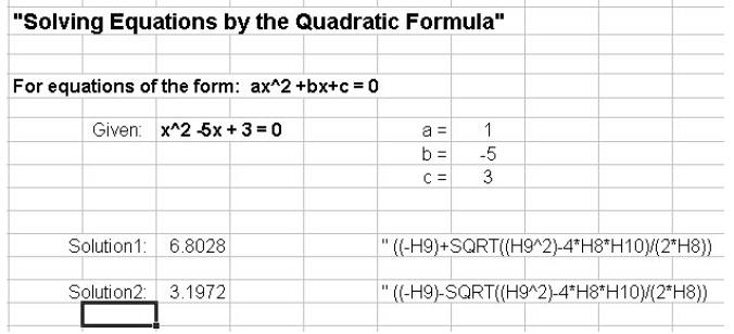
The following example solves equations with the quadratic formula.
Assessment:
• Classwork and homework
Level/Course: Algebra 3/ Trigonometry: This lesson
can be modified to fit any course or
level by changing the problems and answers.
Objective: Students will solve problems and be able to check their
answers.
Activity:
Solve problems (first column) on a scrap sheet of paper, and then type in the
answer in
the cell next to the question (second column). Press enter. If the answer is
right, then
“Correct” will show up in the third column. Work all problems until they are all
Correct.
Example:
| Problem | Answer | ||
| Find the Amplitude | |||
| 1 | y=3sinx | 3 | Correct |
| 2 | y=-2cosx | 2 | Correct |
| Find the Period | |||
| 3 | y=cos3x | 25 | |
| 4 | y=tan2x | 90 | Correct |
| 5 | y=sec2x | 72 |
Example 2:(The numbers in black are the answers to the problem)
| Problem | Answer | ||
| Find the Amplitude | |||
| 1 | y=3sinx | =IF(C3=3,"Correct"," ") | |
| 2 | y=-2cosx | =IF(C4=2,"Correct", " ") | |
| Find the Period | |||
| 3 | y=cos3x | =IF(C6=120,"Correct"," ") | |
| 4 | y=tan2x | =IF(C7=90,"Correct"," ") | |
| 5 | y=sec2x | =IF(C8=180,"Correct"," ") |
Assessment
This use of a spreadsheet for practice with immediate feedback is an efficient
and
effective means of assessment.
Level/Course: Geometry
This lesson fits with convex regular polygons. Learning how to compute and find
relationships between interior, exterior, and central angles is a major concept
in
Geometry. It could also be used when starting the concepts dealing with apothems
of
regular polygons. This lesson is designed for students to see the relationships
between
these different angles.
Objectives:
Given the number of sides on a regular polygon, students will describe
relationships seen
between angles.
Activities:
Enter the number of sides on a regular polygon and see how the angles relate.
Excel will
display the interior, exterior, sum of interior, and central angles of that
polygon.
| Excel Steps : 1. Enter table containing number of sides. 2. Program cells that correspond with each measurement. Example (when A10 is the number of sides): 1 interior angle, =((A10-2)*180)/A10 3. Finish |
Sample Output:
| Number of side, n |
1 interior angle |
1 exterior angle |
total sum of interior angles |
1 central angle |
| 3 | 60 | 120 | 180 | 120 |
| 4 | 90 | 90 | 360 | 90 |
| 5 | 108 | 72 | 540 | 72 |
| 6 | 120 | 60 | 720 | 60 |
| 7 | 128.57143 | 51.428571 | 900 | 51.428571 |
Assessment:
• Individual classwork and homework.
• Provided worksheet.
• Use chart for prediction.
• Writing exercise involving relationships of angles.
Angles in Regular Polygons Worksheet
1. What is always true about the relationship between 1
exterior angle and 1 interior
angle?
2. As 1 interior angle gets bigger what happens to the exterior angle?
3. As the number of sides change, how does the total sum
of the interior angles
change?
4. What is the relationship between 1 interior and 1
exterior angle to the total sum of
interior angles?
5. What is the relationship between 1 interior angle and a central angle?
6. What is the relationship between 1 exterior angle and a central angle?
7. As the number of sides increase, what happens to each interior angle?
Level/Course: Discrete Mathematics
Objective: To solve problems involving permutations and combinations
There are some situations involving choices where the order in which those
choices are
made is important. There also situations where the order is not important.
To find the number of ways n elements can be arranged in order we use
permutation. A
way to help your students to remember that order matters for permutations is the
example
of phone numbers, 555-2163 and 555-2136 are not the same and it matters the
order you
dial the number. Combinations are counting problems where order does not matter.
The
use of card games can help students remember combinations since the order the
cards are
dealt does not change the “hand”.
Activity: Compute Combination: 
Excel Steps:
1. Highlight a cell. (A1)
2. Type in: = combin(10,2)
3. Enter
Activity: Compute Permutation: 
Excel Steps:
1. Highlight a cell. (B1)
2. Type in: = permut(10,2)
3. Enter
Activity: Compute Factorial: 8!
Excel Steps:
1. Highlight a cell. (C1)
2. Type in: = fact(8)
3. Enter
Level/Course: Algebra I or II
The topic of graphing quadratic equations is covered in Algebra I and Algebra
II, but
similar procedures using spreadsheets to examine functions and their graphs
could be
used in more depth in Algebra II.
Objectives: Given a parabolic function, students will be able to predict
features of the
graph based on the sign of the leading coefficient and the value of the
constant. Students
will understand the graphic effect of changing the coefficient of x², the
coefficient of x,
or the constant.
Activities:
Enter the x-values and the function, allowing Excel to compute the y-values.
Create an
xy-scatter plot and add a trendline to display a graph of the parabola. Change
various
signs and values throughout the function to observe the resulting changes in the
graph.
Excel Steps:
1. Enter x-values
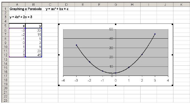
2. Enter the function and direct it to fill in the y-value in the appropriate
cell (ex. If the
first x-value is in cell A6, the function y = 4x² + 2x + 3 would be entered in
cell B6 as
follows: =4*(A6^2)+2*A6+3)
3. Fill in the remaining cells in column B to compute the other y-values (the
function in
B6 can be dragged into the other cells so Excel changes the formula to fill in
A7, A8,
etc.)
4. Choose Chart
5. Select XY (scatter)
6. Finish
7. Chart – Add trendline – (Select polynomial of order 2)
Sample Output:
Assessment:
• Students will graph parabolas without any graphing technology based on the
features of the function discussed
• Students will enter functions into spreadsheets and create graphs to check the
graphs they created
Level/Course: Algebra I
Linear regression is easily accomplished in a spreadsheet in a multiple
representation
format. The data are entered in a table, and the program presents a graphical
and
algebraic representation. The same method works equally well for curve fitting
in
nonlinear functions.
Objectives: Given a set of ordered pairs, students will graph the points,
plot a leastsquares
regression line, and give the equation of the line.
Activities:
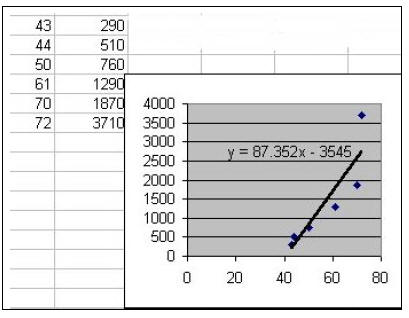
Enter the set of data points, plot them, and then plot a line of best -fit,
called a trendline.
Excel will draw the least - squares regression line and give its equation.
| Excel Steps: 1. Enter x and y data 2. Highlight data 3. Choose Chart 4. Select XY(scatter) 5. Finish 6. Chart - Add trendline - (Select Linear) 7. Options - Display equation on chart. |
Sample Output:
Assessment:
• Individual classwork and homework
• Group Projects with real-world data
• Use of the regression equation for prediction
• Writing exercises involving description of process and reflection on its use
Level/Course: Algebra II
This activity could be used at the introduction of a unit on matrix operations.
Working as
a class or in groups, students could explore how these operations work .
Objectives: Given a matrix, students will learn how to find the scalar
multiple and
determinant of the matrix. With a pair or matrices, students will learn how to
multiply
them.
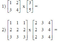
Activities:
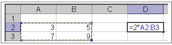
Multiplication by a Scalar
Enter the matrix data and the appropriate equation. Excel will calculate the
matrix ’s
scalar multiple for a given scalar.
| Excel Steps: 1. Enter matrix as it appears in question 2. Several columns over, highlight empty cells the same size as the original matrix 3. Where s is the scalar value, type =s* then highlight the original matrix and the cell values of the original matrix will appear in the equation 4. Press Ctrl-Shift-Enter to finish |
Sample of Procedure:
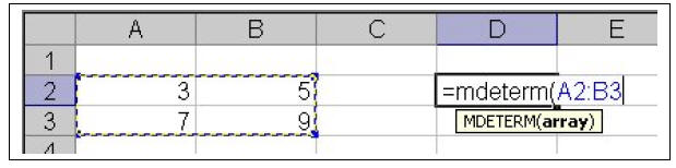
Finding the Determinant
Enter the matrix data and mdeterm(array), the Excel equation for determinants,
then
Excel will calculate the determinant of the matrix.
| Excel Steps: 1. Enter matrix as it appears in the question 2. Several columns over, in an empty cell, type =mdeterm( 3. Highlight the original matrix 4. Type ) to close the parentheses 5. Press Enter or Return to finish |
Sample of Procedure:
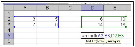
Matrix Multiplication
Enter the data for the two matrices then use Excel equation mmult(array1,array2)
to
multiply the two matrices.
| Excel Steps: 1. Enter first matrix as it appears in the question 2. Several columns over, enter the second matrix 3. Highlight empty cells in the size of the resulting matrix 4. While still highlighted, in one cell type =mmult( 5. Highlight the first matrix 6. Place a comma after the array numbers of the first matrix 7. Highlight the second matrix and end with a parentheses 8. Press Ctrl-Shift-Enter to finish |
Sample of Procedure:
Assessment:
• Group project exploring the algebra behind matrix operations
• Using Excel to perform matrix operations
• Individual class work and homework
• Writing exercises describing discoveries about how matrix operations work
Matrix Operations Worksheet
Using Excel, follow the directions provided in class to perform the following
matrix
operations:
Multiplication by a scalar:
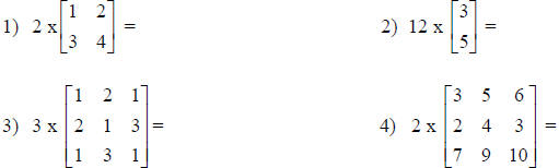
5) How is the solution matrix related to the original
matrix in the problem? What
patterns do you see?
Finding the Determinant:
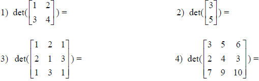
5) What patterns do you see in how the determinant relates
to its’ matrix?
How is the answer for the determinant for the matrix in problem 2 different?
What can you conclude from that?
Matrix Multiplication:
2) What patterns do you see in how the solution relates to
the two original matrices
in the problem 1? How about in problem 2? Can you combine your ideas to make
a general statement for how to multiply any matrices?
Level/Course: Pre-Algebra, Algebra
This activity should be completed by students so that they can see how
real-world
information/data can be put into graphs. This exercise is helpful because it
allows
students not only to see and use real-world data and how it pertains to them,
but students
are also able to utilize their statistical skills to interpret the information
from those
graphs.
Objectives: Given a table of information and data, students will
interpret the given
information and put in into a table. Then, students will be able to put this
information
into any type of graph. These graphs help the students interpret the data and
also to make
conclusions about the given information.
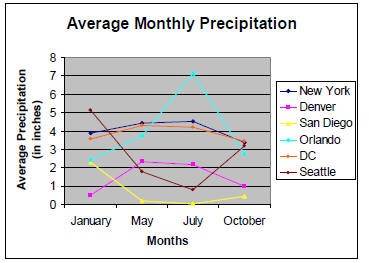
Activities: Gather data from a certain source (i.e. the Internet) and
make a table
organizing the data. Then, plot the data onto a graph. Excel will make the graph
with
various colors, appropriate titles, and a key to help understand the graph.
Sample Output:
| Months | New York | Denver | San Diego | Orlando | DC | Seattle |
| January | 3.88 | 0.51 | 2.28 | 2.43 | 3.57 | 5.13 |
| May | 4.43 | 2.32 | 0.2 | 3.74 | 4.29 | 1.78 |
| July | 4.53 | 2.16 | 0.03 | 7.15 | 4.21 | 0.79 |
| October | 3.39 | 0.99 | 0.44 | 2.73 | 3.43 | 3.19 |
Assessment:
• Individual classwork and homework
• Group projects with real-world data (i.e. Web Quests)
• Written exercises involving a understanding of the graphs and interpretations
of
the given/collected data
Level/Course: Algebra II
Objectives: Given a function and a range of x values, students will use
spreadsheets to
obtain corresponding y values, graph the function, and find the zero ’s of the
function.
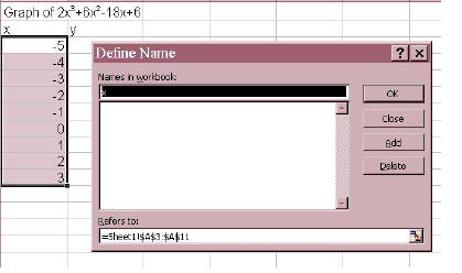
Excel Steps
1. Enter x values
2. Define cells of x values as variables in the given equation.
• Highlight column of x values
• Insert-Name-Define (give variable a name, in this case, x)-OK
4. Graph function
• Highlight x and y values
• Insert-Chart- XY Scatter-Choose appropriate chart type- Finish
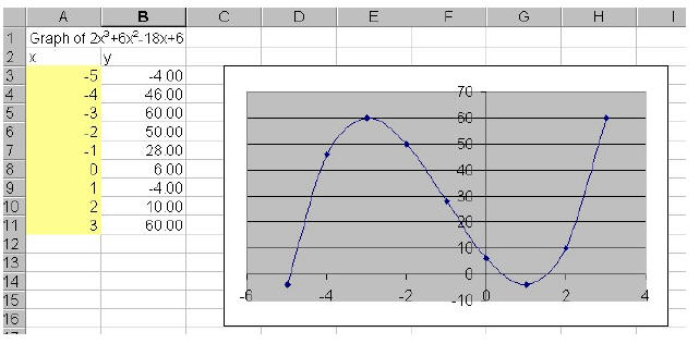
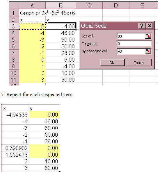
5. From the data and the graph determine approximately
where zero’s occur.
6. Use “Goal Seek” to evaluate function at y=0 to find the values.
• Highlight appropriate y-value cell. (the one before each sign change in y, in
this
case, cells B3, B8, and B9).
• Tools-Goal Seek- Enter 0 in the “To Value” Box, and corresponding
x-value cell
name in the “By Changing Cell” Box – OK
Level / Course: Advanced Placement Statistics or
Discrete Mathematics or Statistics
Objectives:
Statistics involves many calculations that once understood are easily calculated
using
technologies. Technologies used typically include a TI-83 calculator, MiniTab,
Fathom,
or SPSS. Often overlooked for this same purpose of calculating statistics is
Microsoft
Excel. Excel is more readably available in the real world, hence why not teach
students to
use Excel to perform statistical procedures?
Activities:
See attached sheets for some sample outputs from Excel. These are just a few of
the
many calculations Excel will perform. For more commands, the “HELP” feature of
Excel
is great when you type in ‘statistics.’
Statistical Test:
To perform statistical procedures such as t-test and z-test you will first need
to load the
data analysis package.
*Note that this is preloaded on some, to check click on “TOOLS” on the menu bar.
If you
see DATA ANALYSIS (and you can select it) you’re ready to go. If not, under the
TOOLS menu, cluck on “ADD INS” and select the “Analysis Took Pak” and then
load.*
The following is one of many statistical tests Excel will perform.
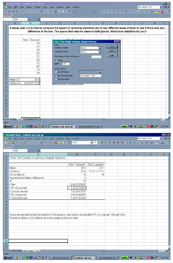
To perform a two-sample t-test (or z-test, depending on if you are dealing
with a
population or a sample):
• Click on “Tools” from the menu bar
• Select “Data Analysis”
• Choose the appropriate statistical test, t-test or z-test. (I used t-test: two
sample unequal
variances assumed.)
• Enter the appropriate columns of data in the first two boxes. (Again you can
use a colon
to indicate a series in a row or column.) IMPORTANT NOTE: You must enter the
first
cell in these boxes as the cell above or before your first actual number! (see
pictures
below)
• For Hypothesized Mean Difference enter 0.
• If you have given your data sets labels, click show labels.
• Click Ok!
• Your statistical test will appear as another worksheet on the tabs below.
Below are the screenshots of my two sample, unequal variance t-test:
Excel commands for Statistical Procedures:
Basics:
| Statistical Procedure | Excel Input |
| Average or MEAN of a given set of data. Assuming the data is entered in a row or column. |
=average(first cell with entry : last cell with entry) |
| Standard Deviation of an entire population | =stdevp(first cell : last cell) |
| Standard Deviation of a sample from a larger population |
=stdev(first cell : last cell) |
Pertaining to the Cumulative Distributive Function (CDF):
| Statistical Procedure | Excel Input |
| Standardize a value, x. | =standardize(x, mean, standard deviation) |
| The Cumulative Distributive Function of a standardized z-score. |
=normsdist(z) |
| The inverse CDF, given a probability (or proportion). |
=normsinv(probability) |
| X< (area to the left) | =normdist(x, mean, standard deviation, True) |
| X> (area to the right) | =1-normdist(x, mean, standard deviation, True) |
| # > X > # (area in-between two values, specifically “high” and “ low ” |
=(normdist(high, mean, standard deviation, True) – normdist(low, mean, standard deviation, true)) |
For a Chi-Squared Statistic:
| Statistical Procedure | Excel Input |
| Chi-Squared distributive value of “chi” | =chidist(chi, degrees of freedom) Note: Degrees of freedom=(number of columns – 1)*(number of rows -1) |
| Prev | Next |