Projection Methods for Linear Equality Constrained Problems
Projection Methods for Linear Equality Constrained Problems
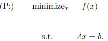
4 Solving the Direction -Finding Problem (DFP)
Approach 1 to solving DFP: solving linear equations
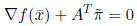
Create the system of linear equations:

and solve this linear system for by any method at your disposal.
If  , then
and so![]() is a Karush-Kuhn-Tucker point of P.
is a Karush-Kuhn-Tucker point of P.
If  , then rescale the solution as follows :
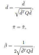
Proposition 4.1  defined above satisfy (1), (2), (3), (4), and (5).
Note that the rescaling step is not necessary in practice,
since we use a
line-search.
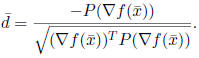
Approach 2 to solving DFP: Formulas
Let
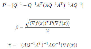
If
![]() > 0, let
> 0, let
If
![]() =0, let
=0, let
![]() =0.
=0.
Proposition 4.2 P is symmetric and positive semi-definite. Hence
![]() ≥ 0.
≥ 0.
Proposition 4.3 ![]() defined above satisfy (1), (2), (3), (4), and (5).
defined above satisfy (1), (2), (3), (4), and (5).
5 Modification of Newton’s Method with Linear
Equality Constraints
Here we consider the following problem:
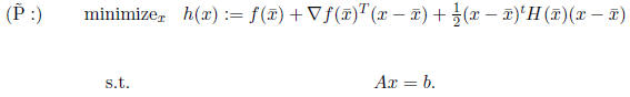
Just as in the regular version of Newton’s method, we
approximate the
objective with the quadratic expansion of f(x) at
![]() :
:
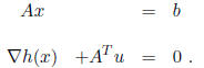
Now we solve this problem by applying the KKT conditions,
and so we
solve the following system for (x, u):
Now let us substitute the fact that:
 and
and
![]() .
.
Substituting this and replacing
![]() , we have the system:
, we have the system:
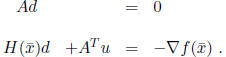
The solution (d, u) to this system yields the Newton
direction d at ![]() .
.
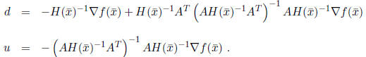
Notice that there is actually a closed form solution to this system, if we
want to pursue this route. It is:
This leads to the following version of Newton’s method for
linearly
constrained problems:
Newton’s Method for Linearly Constrained Problems:
Step 0 Given x0 for which Ax0 = b, set k ← 0
Step 1![]() ← xk.
Solve for
← xk.
Solve for  :
:

If  , then stop.
Step 2 Choose step-size αk =1.
Step 3 Set  Go
to Step 1.
Go
to Step 1.
Note the following:
• If ![]() , then
, then
![]() is a KKT point. To
see this, note from Step 1
is a KKT point. To
see this, note from Step 1
that 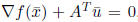 , which are precisely the KKT conditions
for
, which are precisely the KKT conditions
for
this problem.
• Equations (8) are called the “ normal equations ”. They were derived
presuming that  is positive-definite, but can
be used even when
is positive-definite, but can
be used even when
is not positive-definite.
• If is positive definite , then
![]() is a descent
direction. To see this,
is a descent
direction. To see this,
note that  from(8) since
is positive
from(8) since
is positive
definite.
6 The Variable Metric Method
In the projected steepest descent algorithm, the direction d must lie in the
ellipsoid
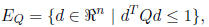
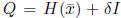
where Q is fixed for all iterations. In a variable metric
method, Q can
vary at every iteration. The variable metric algorithm is:
Step 1.
![]() satisfies
satisfies
![]() Compute
Compute
 .
.
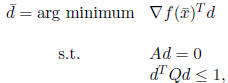
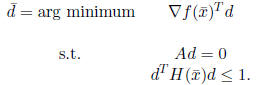
Step 2. Choose a positive-definite symmetric matrix Q. (Perhaps

, i.e., the choice of Q may depend on the current point.) Solve the
direction-
finding problem (DFP):
DFP:
If
![]() , stop. In the case,
, stop. In the case,
![]() is a KKT point.
is a KKT point.
Step 3. Solve
![]() for the stepsize
for the stepsize
![]() , perhaps chosen by an
exact
, perhaps chosen by an
exact
or inexact linesearch.
Step 4. Set
![]() Go to Step 1.
Go to Step 1.
All properties of the projected steepest descent algorithm still hold here.
Some strategies for choosing Q at each iteration are:
• Q = I
• Q is a given matrix held constant over all iterations
• Q =![]() where H(x)
is the Hessian of f(x). It is easy to show
where H(x)
is the Hessian of f(x). It is easy to show
that that in this case, the variable metric algorithm is equivalent to
Newton ’s method with a line-search, see the proposition below.
•  , where
  is chosent to be large for early iterations,
but is chosen to be small for later
iterations. One can think of this
strategy as approximating the projected steepest descent algorithm in
early iterations, followed by approximating Newton’s method in later
iterations.
Proposition 6.1 Suppose that Q =
![]() in the variable
metric algorithm.
in the variable
metric algorithm.
Then the direction ![]() in
the variable metric method is a positive scalar times
in
the variable metric method is a positive scalar times
the Newton direction.
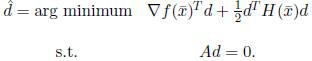
Proof: If Q = ![]() ,
then the vector
,
then the vector ![]() of
the variable metric method is
of
the variable metric method is
the optimal solution of DFP:
DFP:
The Newton direction
![]() for P at the point
for P at the point![]() is the solution of the following
is the solution of the following
problem:
NDP:
If you write down the Karush-Kuhn-Tucker conditions for
each of these two
problems, you then can easily verify that  for some scalar γ> 0.
q.e.d.
| Prev | Next |