Matlab Basics for Math 283
Starting up matlab:
Go to finder -> applications -> matlab701 -> matlab7.01
From a terminal command prompt:
matlab (display matlab desktop, access editor, helpdesk)
matlab –nojvm (no java virtual machine, no desktop -- faster)
matlab –nodisplay (no desktop, no plot windows -- faster)
matlab –help (to see all options)
NOTE: ">>" is the matlab prompt.
Operators, Punctuation
Operators
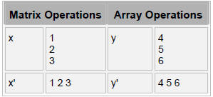
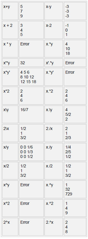
Arithmetic operators in matlab:

follow the convention in linear algebra . Matrices must have correct dimensions
for any
operation. Follows order of operations . Use parentheses to change precedence
>> 1*2/3+4^5-4^5
ans =
0.6667
Element-by-element operators operate on arrays or matrices by element
(essentially
operator preceded by a period):
>> [1 2 3].*[1 2 3]
ans =
1 4 9
Matlab Punctuation
| % | Denotes comment line. Information after % is
ignored by matlab. >> %nothing happens >> |
| , | Comma works like blank space. Concatenates array
elems along row. Shows results. >> x=[1,2,3], x = 1 2 3 |
| ; | Concatenates array elements along column.
Suppresses printing contents of variable to screen. >> x=[1;2;3] x = 1 2 3 >> x=[1;2;3]; >> |
| : | Specifies a range of numbers. A colon in an array
dimension accesses all elements in that dimension. >> z=[1:0.25:2; 3:0.25:4] % row 1: 1 to 2, row 2: 3 to 4, step size/increment by 0.25 z = 1.0000 1.2500 1.5000 1.7500 2.0000 3.0000 3.2500 3.5000 3.7500 4.0000 >> z(:,2) %all rows, column 2 ans = 1.2500 3.2500 >> z(1,:) %all columns, row 1 ans = 1.0000 1.2500 1.5000 1.7500 2.0000 |
| ’ | Apostrophe at the end of a vector or matrix gives
its transpose. >> z(:,2)' ans = 1.2500 3.2500 |
More basic operators/functions

Basic Data Structures
Basic data constructs are arrays and matrices.
Arrays can be row vectors (1 by n array) or column vectors (n by 1 array).
A matrix can have two dimensions (example: m rows and n
columns). Multi-dimensional
arrays can also be specified.
>> row_vect = [1 4 5];
>> column_vect = [1;4;5];
Concatenate column vectors along same row:
>> two_column_vect = [column_vect column_vect]
two_column_vect =
1 1
4 4
5 5
Concatenate row vectors along same column:
>> two_row_vect = [row_vect; row_vect]
two_row_vect =
1 4 5
1 4 5
Accessing array elements
| a(i) | i-th element of array a. |
| A(i , : ) | i-th row of a matrix A, all columns (Can
select certain columns by putting an array of indices instead of ‘:’ ). |
| A(:, i ) | i-th column of a matrix A, all rows (Can
select certain rows also by putting an array of indices instead of ‘:’ ). |
| A(i , j ) | Element in i-th row, j-th column of matrix A. |
Array building
| zeros, ones | Builds arrays with all 0’s or all 1’s
respectively. >> x = zeros(1,3) x = 0 0 0 |
| eye | Creates an identity matrix. >> x= eye(2,2) x = 1 0 0 1 |
Some basic functions on arrays and matrices
Type ‘help function_name’ for details on usage.

Not covered: cell arrays.
File and Workspace Management, File I/O
File and workspace management
| dir, ls | Show files in active directory |
| delete filename | Remove file filename in active directory. |
| cd, pwd | Show present directory |
| cd dir | Changes the directory to dir |
| clear | Remove all variables from workplace |
| clear x | Remove variable x from the workplace. |
| who | List all variables in the workspace |
File I/O
| load | Syntax: load filename Load from file. Check out variations of use. File should have correct format (Same number of columns for each row, rows for each column) and no nonnumeric characters. For instance if you have a file called test.dat in current dir: >> load test.dat >> test test = 1 2 3 |
| save | Syntax: save filename variable –ascii Saves ‘variable’ in ASCII format in’filename’. >> save test_copy.dat test -ascii |
Control Flow
Conditional Control – if , else, elseif, and switch/case
if, else, and elseif
if evaluates a logical expression and executes a group of
statements based on the value
of the expression. In its simplest form , its syntax is
if logical_expression
statements
end
The else and elseif statements further conditionalize the if statement
The else statement has no logical condition . The
statements associated with it execute if
the preceding if (and possibly elseif condition) evaluates to logical 0 (false).
The elseif statement has a logical condition that it
evaluates if the preceding if (and
possibly elseif condition) is false. The statements associated with it execute
if its
logical condition evaluates to logical 1 (true). You can have multiple elseif
statements
within an if block.
For some value of n :
if n < 0 % If n negative, display message.
disp(’Input negative’);
elseif n == 0 % If n equals zero
disp(’Input zero’);
else %n greater than zero is remaining case
disp(’Input positive’);
end
switch, case, and otherwise
switch executes certain statements based on the value of a
variable or expression.
Its basic form is
switch expression (scalar or string)
case value1
statements % Executes if expression is value1
case value2
statements % Executes if expression is value2
.
.
otherwise
statements % Executes if expression does not
% match any case
end
Loop control – for, while, break
for
The for loop executes a statement or group of statements a
predetermined number
of times. Its syntax is
for index = start:increment:end
statements
end
The default increment is 1. You can specify any increment,
including a negative one .
For positive indices, execution terminates when the value of the index exceeds
the
end value; for negative increments, it terminates when the index is less than
the end
value.
For example, this loop executes five times.
x=[1:10];
for n = 2:6
x(n) = 2 * x(n);
end
while
The while loop executes a statement or group of statements
repeatedly as long as
the controlling expression is true (1). Its syntax is:
while expression
statements
end
If the expression evaluates to a matrix, all its elements
must be 1 for execution to
continue. To reduce a matrix to a scalar value, use the all and any functions.
Increments n from 0 to 10:
n = 0;
while n < 10
n = n + 1
end
Exit a while loop at any time using the break statement.
Useless example that
breaks at n==5:
n = 0;
while n < 10
n = n + 1;
if n ==5, break, end
end
Simple Plots
Basic commands
| plot | Draws plot of two equal-sized vectors x,y. Style
is specified by character string s where s could be for example ‘b*’ for blue asterisk or ‘bd’ for blue diamonds representing points. Default is blue line with points connected. Usage: plot(x,y) or plot(x,y, s) |
| hist | Draws histogram of input array. Default number of
bins is 10. Usage: hist(array) or hist(array, num_bins) |
| xlabel | Label for x-axis. Usage: xlabel(’x axis variable’) |
| ylabel | Label for y-axis. Usage: xlabel(’y axis variable’) |
| axis | Set specified x- and y-axis limits. Usage: axis([xmin xmax ymin ymax]) |
| xlim | Set x-axis limits only. Usage: xlim([xmin xmax]) |
| ylim | Set y-axis limits only. Usage: ylim([ymin ymax]) |
| title | Title over plot. Usage: title(’plot title’) |
| hold on, off |
‘hold on’ causes subsequent plots to be
superimposed on current one, whereas ‘hold off’ specifies each new plot start afresh. Default is off. |
| figure | Creates a new figure window. Usage: figure; |
Saving plots
Save plots in desired format using the figure window (File -> Save as) . To save
the plot
on the current figure window as a png file using the command line,type:
>>print( gcf , '-dpng', '-r0', 'plot_filename');
More plotting function examples
Type ‘help function_name’ for details on usage.

Scripts and Functions
An M-file is a text file that contains MATLAB commands and
has a .m filename extension.
Use Matlab Editor/Debugger or any text editor (emacs, vi) to create function.m
or
script.m file. To start in MATLAB, go to File->New-> M-file
Note that the name of the function or script filename is identical to the
command invoked
at MATLAB prompt (without the .m extension).
Script M-files No input or output arguments and operate on variables in
the workspace.
Just a series of commands. Example: script.m
>> x = [-3:.1:3];
>> y = x .^ 2;
>> plot(x,y);
>> xlabel('x');
>> ylabel('y');
>> title('parabola y = x^2');
>> print(gcf,'-dpng','-r0','parabola.png');
>> print(gcf,'-depsc','parabola.eps');
% script.m
% series of matlab commands in a file.
x = [1:10]
mean(x)
Function M-files Contain a function definition line
and can accept input arguments and
return output arguments, and their internal variables are local to the function
(unless
declared global). Syntax requires the first line to be of form:
function [out1, …, outN] = func_name(in1, …, inN)
Example: stats_wrapper.m
function [mean_x, var_x] = stats_wrapper(x)
%stats_wrapper.m
%computes the mean and variance of array x
mean_x = mean(x);
var_x = var(x);
Example usage:
>> [m,v]= stats_wrapper([1,2,3,4,5])
m =
3
v =
2.5000
Statistics in Matlab
Examples:
Some CDF, PDF, Inverse functions, Random number generators
normcdf Normal (Gaussian) cdf given value and
parameters
poisscdf Poisson cdf given value and parameters
binopdf Binomial pdf given value and parameters
geopdf Geometric pdf given value and parameters
norminv Normal (Gaussian) critical values given p and parameters
poissinv Poisson critical values given p and parameters.
normrnd Normal (Gaussian) random numbers given parameters
poissrnd Poisson random numbers given parameters.
Some Hypothesis Tests
ranksum Wilcoxon rank sum test
signrank Wilcoxon signed rank test
signtest Sign test for paired samples
ttest One sample t-test
ttest2 Two sample t-test
ztest Z-test
help function_name
Best way to know how to correctly use built-in function
and understand what it is
doing.
Sources:
1. Highham, D.J., and Higham, N.J. Matlab Guide. SIAM,
Philadelphia, 2000.
2. Martinez, W.L., and Martinez, A.R. Appendix A, Computational Statistics
Handbook With Matlab.
Chapman&Hall/CRC, New York, 2002.
Exercises:
Generate values from a binomial distribution
% Generate 10,000 random values from a binomial
distribution and store in row vector
% empirical_bino. Use help to figure out input values for binornd.
>>empirical_bino = binornd(100,1/2,1,10000);
%Check that the mean and variance are close to that of the
distribution from which it was
% generated.
>> mean(empirical_bino)
>> var(empirical_bino)
% Since binomial with p=1/2 is symmetric, check that median is also near true mean.
>> median(empirical_bino)
% Check out the distribution of the values in
empirical_bino by plotting the histogram.
% Default number of bins is 10.
>>hist(empirical_bino)
% Use hold on to draw/trace plot of the distribution over the histogram.
>>[frequency, bins] = hist(empirical_bino);
>>hold on;
>>plot(bins, frequency, ’b*’); %use blue asterisk
>>xlabel(’bins’);
>>ylabel(’counts’);
>>title(’Simulated distribution’);
>>binsize=bins(2)-bins(1);
>>plot(0:100, 10000*binsize*binopdf(0:100, 100, 1/2),’r’);
What does it look like?
% Working with the cdf
% Get the probability that values from B(0,1) are less than or equal to the mean
% of the values in empirical_bino. Do the same for the median.
% First, check what we know
>> binocdf(50,100,1/2)
>> pmean = binocdf(mean(empirical_bino), 100,1/2)
>> pmedian = binocdf(median(empirical_bino), 100,1/2)
% Use the cdf to get back the critical values
% corresponding to those probability cutoffs
% First, check what we know
>> binoinv(0.5, 100,1/2)
>> binoinv(pmean, 100,1/2)
>> binoinv(pmedian, 100,1/2)
% Plot the cdf of empirical_bino
% Need to sort the values in empirical_bino from low to high and
% get the corresponding probability Px = P(X<=x) for each value in the
% array according to the theoretical distribution.
>> Px = binocdf(sort(empirical_bino), 100,1/2);
% Use Figure to create a new window
>>figure;
% Plot the sorted values of empirical_bino on x-axis and
% corresponding theoretical probabilities on y-axis.
>>plot(sort(empirical_bino), Px)
>>xlabel(’x’)
>>ylabel(’P_x’);
>>title(’cdf of empirical bino’);
Odds and Ends
%because we can let us practice file i/o with pmean
>> save pmean_file pmean –ascii
>> load pmean_file
>> pmean_file
>> delete pmean_file
Function example
Create simple function called sim_bino.m that plots the distribution of m values
generated
from a binomial distribution with parameters n and p and returns the mean and
variance
of the observed distribution
% Calls sim_bino with parameters n=100, p=1, m=100000 and
saves plot as test.png
% Note that the character string ‘test’ is in single quotes
>>[obs_mean, obs_var] = sim_bino(100,1/2,10000, ’test’)
File: sim_bino.m
function [obs_mean, obs_var] = sim_bino(n, p, m, plotname)
%sim_bino.m
%----------------
% Simple function that plots distribution of m values from a binomial
distribution with
% parameters n and p and saves this plot in PNG as ‘plotname’ in the current
directory.
empirical_bino = binornd(n, p, 1, m);
figure;
hist(empirical_bino);
[frequency, bins] = hist(empirical_bino);
hold on;
plot(bins, frequency, ’b-*’); %use blue line and asterisk
xlabel(’bins’);
ylabel(’counts’);
title(’Simulated distribution’);
%save plot as plotname.png
print(gcf, '-dpng', '-r0',plotname);
obs_mean = mean(empirical_bino);
obs_var = var(empirical_bino);
| Prev | Next |