Graphing Linear Inequalities

Section 3.1 Graphing Systems of Linear Inequalities in Two Variables

Graphing Linear Inequalities .

1. Graph the boundary line.
a. Replace the inequality sign with an equal sign, and graph the equation obtained .
This means that you are graphing a line (the boundary line).
b. Note: Use a dashed/dotted line if the problem involves a strict inequality, < or >.
Otherwise use a solid line, indicating that the line itself is part of the solution.

Example 1: To make sure that you are graphing the correct line and/or shading the
correct region, be sure you can solve for y correctly . In the problems below, the
boundary line is identified, and then the equation solved for y. Note: It is not necessary to
simplify the equation into a formal format if you are using your calculator to graph it.

3x −5y ≤14 Boundary line: 3x − 5y = 14 Solving for y:

− 2x + 7 y ≤ 21 Boundary line: − 2x + 7y = 21 Solving for y: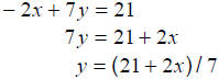

8x ≤ 4y − 3 Boundary line: 8x = 4y − 3 Solving for y: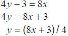

Once the boundary line equation is in y = form for graphing, the line should be graphed,
and THEN the decision must be made about which side of the line to shade.

If you don’t graph with the calculator, try choosing 2 values for x and running each one
through the equation for a corresponding y-value. Plot the two points . Draw the line.

2. Shade the appropriate half-plane.

Method 1 (regular shading – not reverse shading):
a. Pick a test point (the origin is convenient, if possible) lying in one of the half planes
determined by the line. Substitute the values of x and y into the given inequality.
b. If the inequality is satisfied, shade the half-plane containing the test point.
Otherwise, shade the other half-plane.

Again, a re-cap of the process described above: using a test point is one way to make
the decision about shading. Look at the graph of your line, and choose a point (x, y)
that you are sure is not on the line. Test it in the original inequality (Don’t test it in the
equation of the line; it will never work there!). If the result is true, then shade the side
of the line where your test point lies. If the result is false, then shade the side of the
line opposite where your test point lies.

Method 2 (regular shading – not reverse shading):
a. Solve the original inequality for y, making sure to follow all rules for manipulating
inequalities. (or “visually” examine the inequality from a “ positive y perspective ”)
b. For > or ≥ shade above the line; for < or ≤ shade below the line.
(for vertical lines, < is to the left and > is to the right)

Further comments on the process described above: this approach allows you to
reformat for graphing of the line while simultaneously manipulating the inequality so
that you can observe the direction of the inequality sign for shading. This approach
requires great care, since dividing or multiplying by a negative value requires reversing
the inequality sign.

Once you solve for y with the inequality still in place, then you should be accurately
looking at the inequality from the “positive y perspective”. In that case, < or ≤ should
indicate to shade below the line, and > or ≥ should indicate to shade above the line.

Visual examination of the original inequality from a “positive y perspective” is another
way to make the decision about shading. However, it is NOT always as simple as “> or
≥ means shade above” and “< or ≤ means shade below”. If you are reading the sign
from the “positive y perspective” then it is that simple.

Shade below the line:
Shade below the line:

Example 2: Try analyzing the inequalities below from a “positive y perspective”. If the
y- term is negative ( or subtracted ), visualize adding the y-term to both sides of the
inequality, so that the y-term is positive (thus a “positive y perspective”).

In these examples, would you shade “above” or “below” the boundary line?

Horizontal and Vertical lines. Horizontal lines (y = b) and vertical lines (x = a) have
some unique properties . Since vertical lines cannot be written in a “y = “form, they are not
easily graphed on a graphing calculator. Be sure you recognize vertical lines by their
equations, so that you can hand-graph them, and shade the appropriate side of a related
inequality (such as x ≤ 2).

Example 3: Graph the solution set for each inequality below:

Example 4: Graph the solution set for each inequality below:

Graphing Systems of Linear Inequalities

The solution set of a system of linear inequalities in x and y is the set of all points
(x, y) that satisfy each and every inequality in the system.

The solution set of a system of linear inequalities is bounded if it can be enclosed by a
circle . Otherwise it is unbounded.

Graphing steps:
For each inequality in the system repeat steps 1 & 2 in the notes for graphing linear
inequalities. Then…

3. Mark the area of intersection.
a. Observe the area where all the inequalities in the system overlap in shading.
This area is your solution to the system.
b. Outline the area, shade darkly, or whatever it takes to make the answer obvious.

Reverse shading.
1. Reverse shading is a technique that can be useful when 3 or more non-trivial
inequalities are involved.
2. Reverse shading is a technique where you shade the non-solution areas for each
inequality in the problem, understanding that the solution will then be the area that has
NO shading rather than the area with ALL the overlapping shading.
3. If you use reverse shading, it is even more important that you make your intended
answer obvious. Outline the area, and label it!
4. Reverse shading is not assumed! It is a optional technique.
If you use reverse shading, state that you have done so, AND mark your answer well.

Example 5: Graph the solution set for the system.

Example 6: Graph the solution set for the system.

bounded? or unbounded?

Example 7: Graph the solution set for the system.

Illustrate with regular shading.	Illustrate with reverse shading.

…bounded or unbounded?...