A Brief Introduction to Matrix Operations

A matrix is usually defined as an array of numbers that may be treated as an algebraic
object. Usually we refer to a number (m) of horizontal rows and (n) vertical columns.
The dimensionality of the matrix is given by m×n. A vector is a special case with only a
single column or row. A column vector is a 1×n matrix.

A common type of operation is already familiar to you. Consider 3 equations in 3
unknowns

This system can be readily solved to find the values of x , y and z. It an also be written in
matrix form as

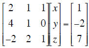
where the unknown scalar terms (x, y and z) are

collected into a column vector x. Sometimes vectors are written with an arrow overbar,
sometimes in bold type. In this case the 3×3 matrix A is often called the coefficient
matrix. If there are as many equations as unknowns A will be square.

The rules for multiplying a matrix and a column include:
1 dimension must be the same, and the operations proceed element by element.
We multiply two vectors to produce a the “inner product”:

Multiplication of a 3×3 matrix by a 1×3 column vector is done one row at a time:

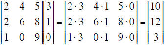
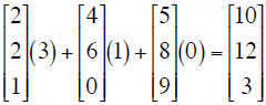
An easy way to do this calculation is by treating each element of the column
vector as a scalar and multiplying each column of the square matrix, then summing to get
the resultant column vector:

Note: for matrices, the associative law holds: A× (C×D) = (A×C) ×D but not the
commutative law: A×B ≠ B×A. It is also useful to define the identity matrix I:

where any matrix B×I = B. Yu can easily check this.

Now, back to the system of 3 equations in 3 unknowns. To solve it, we would
normally
subtract 2 times the first equation from the second, then
subtract -1 times the first equation from the third, then
subtract -3 times the second equation from the third

The multipliers used (2, -1, -3) are known as pivots.

In matrix form the process is known as Gaussian elimination , and we would end up with

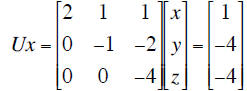
where U is an “upper triangular” matrix.

This system would be easy to solve for x, y, z by back substitution beginning with
z = -4. At the same time there is a matrix L (lower triangular) for which A = LU. In this
case

note that the entries below the diagonal are the pivots we

encountered above. The diagonal terms are those of the identity matrix. Decomposing a
matrix into these upper and lower triangular terms is known as “LU factorization”.

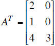
Transpose: this is a common operation, and boils down to exchanging the columns of one
matrix for the rows of another:

If then

For a vectors, a m×1 row vector is transposed to form a 1×n column vector.
In MATLAB, type:

the apostrophe is the tranpose operator

Inverse: the inverse of a matrix is of great importance. For a matrix A, we often write the
inverse as A^-1. A matrix has an inverse if A × A^-1= I. The matrix inverse is usually found
by the Gauss-Jordan method. Any linear algebra textbook will give the algorithm, which
is a simple extension of the pivot technique.

Why do we care about the inverse of a matrix?

One reason is that a fundamental operation in numerical computation is solution of
systems of equations of the form Ax=b for the vector of unknowns x. A solution is:

x = A^-1b so the inverse of A holds the key to the solution.

In MATLAB

(I used the transpose operator to save typing 3 different rows. Instead, I typed 1 row with 3 columns and then transposed it to give “b” correctly as a column vector)

and this is the correct solution to our system of 3 equations in 3 unknowns (x=-1, y=2,
z=1). This type of problem is known as an “inverse” problem: if we know the coefficients
for a system (A) and we know the “output” (b) then we can solve for the unknown terms
x by calculating the inverse of A.

There is an easier (and numerically faster) way to do this in MATLAB using the “reverse
division ” operator, \.

This avoids the syntax associated with the matrix inverse, and is actually carried out in
fewer operations and thus less CPU time. Most of the time this won’t matter, but for
some problems it actually does.

Computers solve problems like this with astonishing speed. Numerical methods may be
thought of as a family of techniques designed to represent problems we need to solve,
like our box model equations or a diffusion equation, in terms of simple if highly
repetitive algebra such as the problem Ax=b. Some of the most sophisticated numerical
algorithms for systems of both ordinary and partial differential equations boil down to
expressing the equations in terms of linear or more often non-linear algebraic equations
that can be solved by executing many rapid elementary steps. MATLAB is full of such
features, and we’ll learn to use a few to solve some of the problems we run across.