Quadratic Forms , Critical Points, Principal Axes, and the 2nd Derivative Test

A typical question from multivariable calculus is:

Find all critical points of the function . Determine which give relative maxima, relative minima, or saddle points.

As you recall, we first find the critical points for this function. This gives us:

So, we must have x² - 6x + (2 - 2x) + 13 = x² - 8x + 15 = (x - 3)(x - 5) = 0
These yield the two critical points (3,-4) and (5,-8). The next question is then:

To answer this question, we generally appeal to the 2nd Derivative Test, which can be formulated as follows:

Let f (x, y) be a function which is continuous, with continuous first and second partial derivatives. Define the Hessian matrix to be the (symmetric) matrix consisting of the 2nd partial derivatives, i.e. . Let be a critical point for this function. If , then will give a relative maximum or minimum for this function. If either or , then there is a relative minimum at . If either  or , then there is a relative maximum at . If , then will give a saddle point for this function. If , then there is insufficient information provided by the 2nd derivatives to distinguish between a possible relative maximum, relative minimum, or saddle point at for this function. That is, the 2nd derivative test is inconclusive.

The 2nd Derivative Test is derived from the idea of quadratic approximation. It is easily shown that the quadratic function
that best approximates a given (sufficiently differentiable) function f (x, y) in the vicinity of a point is given by:



If we denote by the (gradient) row vector , and let , and if we further write x = (x, y) and
, then the above expression becomes :

(Verify this!)

At a critical point the situation is much simpler, since . In this case, the quadratic approximation is simply:

where h is small

Thus, the question of whether there is a maximum, minimum, saddle point, or whatever at boils down to our
being able to understand the quadratic form , and, in particular, what its sign is for any h.

Definition: A quadratic form in Rⁿ is a function q(h) of the form q(h) = h^TAh for some symmetric matrix A. In other
words, a quadratic form is just a 2nd degree expression involving the coordinates .

Example: The quadratic function q(x, y, z) = x² + 3y² - 2z² + 7xy - 6yz is a quadratic form. Note that it has neither a
constant term nor any linear terms . You may verify that with and , we have q(x) = x^TAx.

Definition:
A quadratic form q(h) (and its matrix A) is called positive definite if q(h) > 0 for all h ≠ 0.
A quadratic form q(h) is called negative definite if q(h) < 0 for all h ≠ 0.
A quadratic form q(h) is called positive semi-definite if q(h) ≥ 0 for all h ≠ 0.
A quadratic form q(h) is called negative semi-definite if q(h) ≤ 0 for all h ≠ 0.
A quadratic form q(h) is called indefinite if q(h) takes on both positive and negative values.

The most important fact that we’ll need is the:

Given a quadratic form q(h) = h^TAh, with A symmetric, there is a orthonormal basis of eigenvectors
of A, an orthogonal matrix P whose columns are the vectors of B, and P^-1AP = P^TAP = D, a diagonal matrix whose
diagonal entries are the (real) eigenvalues of A. Thus A = PDP^T and, if we define we have:

In this form, it is easy to see that:

A quadratic form q(h) is positive definite if all eigenvalues of A are strictly positive.
A quadratic form q(h) is negative definite if all eigenvalues of A are strictly negative.
A quadratic form q(h) is positive semi-definite if all eigenvalues of A are either positive or zero.
A quadratic form q(h) is negative semi-definite if all eigenvalues of A are either negative or zero.
A quadratic form q(h) is indefinite if some of the eigenvalues of A are positive and some are negative.

From this, we conclude:

2nd Derivative Test (second form): A critical point for a function f (x) will give: (1) a relative minimum if all eigenvalues of the Hessian matrix are strictly positive. (2) a relative maximum if all eigenvalues of the Hessian matrix are strictly negative. (3) neither a relative maximum nor a relative minimum if some of the eigenvalues of are positive and some are negative. (4) Further analysis is necessary in the case where the Hessian matrix is positive semi-definite (a relative minimum or neither) or negative semi-definite (a relative maximum or neither).

The reasoning behind (4) is simply that the second derivative test is based on a quadratic approximation and in the
borderline case where an eigenvalue is zero , we cannot rely on this approximation to make any valid conclusions.

Notice that for a function of two variables , in cases (1) and (2) the determinant of the Hessian matrix will be the product of
the two eigenvalues and will be positive. In the case where both eigenvalues are positive, the trace of the Hessian matrix
(the sum of its diagonal terms = the sum of its eigenvalues) will be positive and hence either or must be positive. In
the case where both eigenvalues are negative, the trace of the Hessian will be negative and hence either or must be
negative. In case (3) for a function of two variables, the determinant will thus be negative. In case (4), the determinant will
be zero. These observations yield our earlier version of the 2nd derivative test.

This second version of the second derivative test actually tells us quite a bit more. It tells us that there is a new coordinate
system defined in the vicinity of a given critical point, based on the principal axes, in which

This tells us, in particular, that, in the vicinity of this critical point, changes in the function will be most sensitive to
changes in the direction of the eigenvector associated with the eigenvalue of largest magnitude.

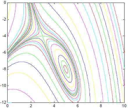
In conclusion, here’s an unlabeled contour diagram for the function with
its two critical points, a saddle point at (3, -4) with f (3, -4) = 19, and a relative minimum at (5, -8) with .
You may want to carry out the calculations above at each of the critical points to find the associated eigenvalues and
principal axes and relate what you find to the shape of the contours in the vicinity of the relative minimum at (5, -8) and, in
particular, which directions give maximum growth.

Exercises: For each of the following functions, find all critical points and determine, for each critical point, whether it
gives a relative maximum, a relative minimum, or neither. Use eigenvalue analysis to justify your answers. At any
minimum, determine which directions (from the critical point) will produce the fastest incremental increase in the
function’s values per distance. At any maximum, determine which directions (from the critical point) will produce the
fastest incremental decrease in the function’s values per distance.
(Note: Despite the seemingly complicated algebra , you should be able to find all the critical points. Really, I swear.)

#1: f (x, y) = x³ + 22x² + 41y² - 24xy - 176x - 68y + 500
#2: f (x, y, z) = 4x³ - 4y³ -26x² + 21y² - 3z² - 2yz + 56x -30y + 22z