Products and Quotients of Rational Functions

Section 7.4 Products and Quotients of Rational Functions 661

In this section we deal with products and quotients of rational expressions. Before we
begin, we’ll need to establish some fundamental definitions and technique. We begin
with the definition of the product of two rational numbers.

Definition 1. Let a/b and c/d be rational numbers. The product of these rational numbers is defined by or more compactly

The definition simply states that you should multiply the numerators of each rational
number to obtain the numerator of the product , and you also multiply the
denominators of each rational number to obtain the denominator of the product. For
example,

Of course, you should also check to make sure your final answer is reduced to lowest
terms.

Let’s look at an example.

Example 3. Simplify the product of rational numbers

First, multiply numerators and denominators together as follows.

However, the answer is not reduced to lowest terms . We can express the numerator as
a product of primes.

210 = 21 · 10 = 3 · 7 · 2 · 5 = 2 · 3 · 5 · 7

It’s not necessary to arrange the factors in ascending order, but every little bit helps.
The denominator can also be expressed as a product of primes.

2310 = 10 · 231 = 2 · 5 · 7 · 33 = 2 · 3 · 5 · 7 · 11

We can now cancel common factors .

662 Chapter 7 Rational Functions

However, this approach is not the most efficient way to proceed, as multiplying numerators
and denominators allows the products to grow to larger numbers, as in 210/2310.
It is then a little bit harder to prime factor the larger numbers.

A better approach is to factor the smaller numerators and denominators immediately,
as follows.

We could now multiply numerators and denominators, then cancel common factors,
which would match identically the last computation in equation (5).

However, we can also employ the following cancellation rule.

Cancellation Rule. When working with the product of two or more rational expressions, factor all numerators and denominators, then cancel. The cancellation rule is simple: cancel a factor “on the top” for an identical factor “on the bottom.” Speaking more technically, cancel any factor in any numerator for an identical factor in any denominator.

Thus, we can finish our computation by canceling common factors, canceling “something
on the top for something on the bottom.”

Note that we canceled a 2, 3, 5, and a 7 “on the top” for a 2, 3, 5, and 7 “on the
bottom.”

Thus, we have two choices when multiplying rational expressions:

• Multiply numerators and denominators, factor, then cancel.
• Factor numerators and denominators, cancel, then multiply numerators and denom-
inators.

It is the latter approach that we will use in this section. Let’s look at another
example.

Section 7.4 Products and Quotients of Rational Functions 663

Example 6. Simplify the expression

State restrictions.

Use the ac-test to factor each numerator and denominator. Then cancel as shown.

The first fraction’s denominator has factors x − 3 and x + 5. Hence, x = 3 or x = −5
will make this denominator zero. Therefore, the 3 and −5 are restrictions.

The second fraction’s denominator has factors x + 2 and x − 4. Hence, x = −2 or
x = 4 will make this denominator zero. Therefore, −2 and 4 are restrictions.

Therefore, for all values of x, except the restrictions −5, −2, 3, and 4, the left side
of

is identical to its right side.

It’s possible to use your graphing calculator to check your results. First, load the
left- and right-hand sides of equation (8) into the calculator’s into Y1 and Y2 in your
graphing calculator ’s Y= menu, as shown in Figure 1(a). Press 2nd TBLSET and set
TblStart = −6 and ΔTbl = 1, as shown in Figure 1(b). Make sure that AUTO is
highlighted and selected with the ENTER key on both the independent and dependent
variables. Press 2nd TABLE to produce the tabular display in Figure 1(c).

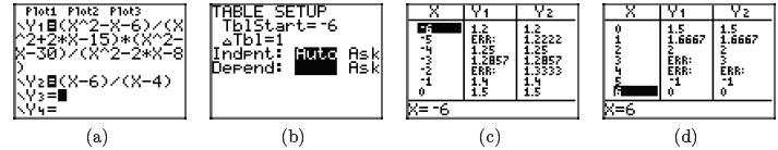
Figure 1. Using the table features of the graphing calculator to check the result in
equation (8).

Remember that the left- and right-hand sides of equation (8) are loaded in Y1 and
Y2, respectively.

664 Chapter 7 Rational Functions

• In Figure 1(c), note the ERR (error) message at the restricted values of x = −5
and x = −2. However, other than at these two restrictions, the functions Y1 and
Y2 agree at all other values of x in Figure 1(c).

• Use the down arrow to scroll down in the table to produce the tabular results shown
in Figure 1(d). Note the ERR (error) message at the restricted values of x = 3 and
x = 4. However, other than at these two restrictions, the functions Y1 and Y2 agree
at all other values of x in Figure 1(d).

• If you scroll up or down in the table, you’ll find that the functions Y1 and Y2 agree
at all values of x other than the restricted values −5, −2, 3, and 4.

Let’s look at another example.

Example 9. Simplify

State any restrictions.

The first numerator can be factored using the difference of two squares pattern .

The second denominator is a perfect square trinomial and can be factored as the square
of a binomial .

You will want to remove the greatest common factor from the first denominator and
second numerator.

and

Thus,

We’ll need to execute a sign change or two to create common factors in the numerators
and denominators. So, in both the first and second numerator, factor a −1 from the
factor 3 − x to obtain 3 − x = −1(x − 3). Because the order of factors in a product
doesn’t matter, we’ll slide the −1 to the front in each case.

We can now cancel common factors.

Section 7.4 Products and Quotients of Rational Functions 665

A few things to notice:

• The factors 3 + x and x + 3 are identical, so they may be cancelled, one on the top
for one on the bottom.

• Two factors of x − 3 on the top are cancelled for (x − 3)² (which is equivalent to
(x − 3)(x − 3)) on the bottom.

• An x on top cancels an x on the bottom.

• We’re left with two minus signs (two −1’s) and a 2. So the solution is a positive 2.

Finally, the first denominator has factors x and x + 3, so x = 0 and x = −3 are
restrictions (they make this denominator equal to zero). The second denominator has
two factors of x − 3, so x = 3 is an additional restriction .

Hence, for all values of x, except the restricted values −3, 0, and 3, the left-hand
side of

is identical to the right-hand side. Again, this claim is easily tested on the graphing
calculator which is evidenced in the sequence of screen captures in Figure 2.

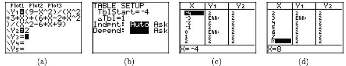
Figure 2. Using the table features of the graphing calculator to check the result in
equation (11).

An alternate approach to the problem in equation (10) is to note differing orders
in the numerators and denominators (descending, ascending powers of x) and anticipate
the need for a sign change. That is, make the sign change before you factor.

For example, negate (multiply by −1) both numerator and fraction bar of the first
fraction to obtain

According to our sign change rule, negating any two parts of a fraction leaves the
fraction unchanged.

666 Chapter 7 Rational Functions

If we perform a similar sign change on the second fraction (negate numerator and
fraction bar), then we can factor and cancel common factors.

Division of Rational Expressions

A simple definition will change a problem involving division of two rational expressions
into one involving multiplication of two rational expressions. Then there’s nothing left
to explain, for we already know how to multiply two rational expressions.

So, let’s motivate our definition of division. Suppose we ask the question, how many
halves are in a whole? The answer is easy, as two halves make a whole. Thus, when
we divide 1 by 1/2, we should get 2. There are two halves in one whole.

Let’s raise the stakes a bit and ask how many halves are in six? To make the
problem more precise, imagine you’ve ordered 6 pizzas and you cut each in half. How
many halves do you have? Again, this is easy when you think about the problem in
this manner, the answer is 12. Thus,

(how many halves are in six) is identical to

6 · 2,

which, of course, is 12. Hopefully, thanks to this opening motivation, the following
definition will not seem too strange.

Definition 12. To perform the division invert the second fraction and multiply, as in

Thus, if we want to know how many halves are in 12, we change the division into
multiplication (“invert and multiply”).

Section 7.4 Products and Quotients of Rational Functions 667

This makes sense, as there are 24 “halves” in 12. Let’s look at a harder example.

Example 13. Simplify

Invert the second fraction and multiply. After that, all we need to do is factor
numerators and denominators, then cancel common factors.

An interesting way to check this result on your calculator is shown in the sequence of
screens in Figure 3.

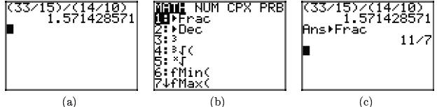
Figure 3. Using the calculator to check division of fractions.

After entering the original problem in your calculator, press ENTER, then press the MATH
button, then select 1:I Frac from the menu and press ENTER. The result is shown in
Figure 3(c), which agrees with our calculation above.

Let’s look at another example.

Example 15. Simplify

State the restrictions.

Note the order of the first numerator differs from the other numerators and denominators,
so we “anticipate” the need for a sign change, negating the numerator and
fraction bar of the first fraction. We also invert the second fraction and change the
division to multiplication (“invert and multiply”).

The numerator in the first fraction in equation (17) is a quadratic trinomial, with
ac = (2)(−9) = −18. The integer pair 3 and −6 has product −18 and sum −3. Hence,

668 Chapter 7 Rational Functions

The denominator of the first fraction in equation (17) easily factors using the difference
of two squares pattern.

The numerator of the second fraction in equation (17) is a quadratic trinomial, with
ac = (2)(−12) = −24. The integer pair −3 and 8 have product −24 and sum 5. Hence,

To factor the denominator of the last fraction in equation (17), first pull the greatest
common factor (in this case x), then complete the factorization using the difference of
two squares pattern.

We can now replace each numerator and denominator in equation (17) with its factorization,
then cancel common factors.

The last denominator has factors x and x − 4, so x = 0 and x = 4 are restrictions.
In the body of our work, the first fraction’s denominator has factors x + 4 and x − 4.
We’ve seen the factor x − 4 already, so only the factor x + 4 adds a new restriction,
x = −4. Again, in the body of our work, the second fraction’s denominator has factors
x, 2x + 3, and 2x − 3, so we have added restrictions x = 0, x = −3/2, and x = 3/2.

There’s one bit of trickery here that can easily be overlooked. In the body of our
work, the second fraction’s numerator was originally a denominator before we inverted
the fraction. So, we must consider what makes this numerator zero as well . Fortunately,
the factors in this numerator are x + 4 and 2x − 3 and we’ve already considered the
restrictions produced by these factors.

Hence, for all values of x, except the restricted values −4, −3/2, 0, 3/2, and 4, the
left-hand side of

Section 7.4 Products and Quotients of Rational Functions 669

is identical to the right-hand side.

Again, this claim is easily checked by using a graphing calculator, as is partially
evidenced (you’ll have to scroll downward to see the last restriction come into view) in
the sequence of screen captures in Figure 4.

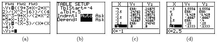
Figure 4. Using the table feature of the calculator to check the result in equation (18).

Alternative Notation. Note that the fractional expression a/b means “a divided
by b,” so we can use this equivalent notation for a ÷ b. For example, the expression

is equivalent to the expression

Let’s look at an example of this notation in use.

Example 21. Given that

and

simplify both f(x)g(x) and f(x)/g(x).

First, the multiplication. There is no possible cancellation, so we simply multiply
numerators and denominators.

This result is valid for all values of x except −3.

On the other hand,

670 Chapter 7 Rational Functions

When we “invert and multiply,” then cancel, we obtain

This result is valid for all values of x except −3 and 0.