Electric Engineer 364a Homework 7 additional problems

Suggestions for exercise 9.30

We recommend the following to generate a problem instance:

n = 100;
m = 200;
randn(’state’,1);
A=randn(m,n);

Of course, you should try out your code with different dimensions, and different data as well.

In all cases, be sure that your line search first finds a step length for which the tentative
point is in domf; if you attempt to evaluate f outside its domain, you’ll get complex
numbers, and you’ll never recover.

To find expressions for f(x) and ²f(x), use the chain rule (see Appendix A.4); if you
attempt to compute 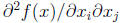, you will be sorry.

To compute the Newton step, you can use vnt=-H\g.

Suggestions for exercise 9.31

For 9.31a, you should try out N = 1, N = 15, and N = 30. You might as well compute and
store the Cholesky factorization of the Hessian , and then back solve to get the search direc-
tions, even though you won’t really see any speedup inMatlab for such a small problem. After
you evaluate the Hessian, you can find the Cholesky factorization as L=chol(H,’lower’).
You can then compute a search step as -L’\(L\g), where g is the gradient at the current
point. Matlab will do the right thing, i.e., it will first solve L\g using forward subsitution,
and then it will solve -L’\(L\g) using backward substitution. Each substitution is order
n^2.

To fairly compare the convergence of the three methods (i.e., N = 1, N = 15, N = 30),
the horizontal axis should show the approximate total number of flops required, and not the
number of iterations. You can compute the approximate number of flops using (n^3)/3 for each
factorization, and 2n^2 for each solve (where each ‘solve’ involves a forward subsitition step
and a backward subsitution step).

Additional exercises

1. Three-way linear classification . We are given data

three nonempty sets of vectors in R^n. We wish to find three affine functions on R^n,

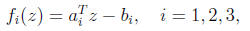
that satisfy the following properties :

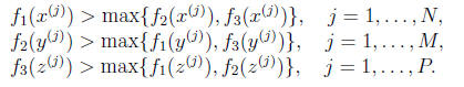
In words: f₁ is the largest of the three functions on the x data points, f₂ is the largest
of the three functions on the y data points, f₃ is the largest of the three functions on
the z data points. We can give a simple geometric interpretation: The functions f₁,
f₂, and f₃ partition R^n into three regions,

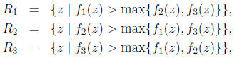
defined by where each function is the largest of the three. Our goal is to find functions
with

Pose this as a convex optimization problem. You may not use strict inequalities in
your formulation .

Solve the specific instance of the 3-way separation problem given in sep3way_data.m,
with the columns of the matrices X, Y and Z giving the x^(j), j = 1, . . . ,N, y^(j), j =
1, . . . ,M and z^(j), j = 1, . . . , P. To save you the trouble of plotting data points and
separation boundaries, we have included the plotting code in sep3way_data.m. (Note
that a1, a2, a3, b1 and b2 contain arbitrary numbers; you should compute the correct
values using cvx .)

2. Efficient numerical method for a regularized least-squares problem. We consider a regularized least squares problem with smoothing,

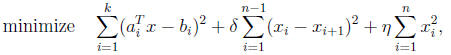
where is the variable , and are parameters.

(a) Express the optimality conditions for this problem as a set of linear equations
involving x. (These are called the normal equations.)

(b) Now assume that k << n. Describe an efficient method to solve the normal
equations found in (2a). Give an approximate flop count for a general method
that does not exploit structure, and also for your efficient method.

(c) A numerical instance . In this part you will try out your efficient method. We’ll
choose k = 100 and n = 2000, and First, randomly generate A and
b with these dimensions. Form the normal equations as in (2a), and solve them
using a generic method. Next, write (short) code implementing your efficient
method, and run it on your problem instance. Verify that the solutions found by
the two methods are nearly the same, and also that your efficient method is much
faster than the generic one.

Note: You’ll need to know some things about Matlab to be sure you get the speedup
from the efficient method. Your method should involve solving linear equations with
tridiagonal coefficient matrix. In this case, both the factorization and the back sub-
stitution can be carried out very efficiently. The Matlab documentation says that
banded matrices are recognized and exploited, when solving equations, but we found
this wasn’t always the case. To be sure Matlab knows your matrix is tridiagonal, you
can declare the matrix as sparse, using spdiags, which can be used to create a tridiagonal
matrix. You could also create the tridiagonal matrix conventionally, and then
convert the resulting matrix to a sparse one using sparse.

One other thing you need to know. Suppose you need to solve a group of linear
equations with the same coefficient matrix, i.e., you need to compute
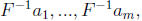
where F is invertible and a_i are column vectors. By concatenating columns, this can
be expressed as a single matrix

To compute this matrix using Matlab, you should collect the righthand sides into one
matrix (as above) and use Matlab’s backslash operator: F\A. This will do the right
thing: factor the matrix F once, and carry out multiple back substitutions for the
righthand sides.