Engineering Mathematics I
1. The Second Mid-Term covers Chapter 9 (nonlinear
differential equations
and stability), Chapter 6 (Laplace Transform), and Chapter 5
(Series Solutions). Materials previously covered in Mid-Term #1 are
assumed known (e.g. direction fields, undetermined coefficients, integration
factor, . . . ).
2. Chapter 9, Nonlinear differential equations and stability. This
is the fun chapter. The basic ideas are presumably good for more than
two variables , but the most successful applications of the basic ideas
are for two variable problems . (Remember, there is no chaos in two-dimensional
problems).
• What does “autonomous” mean? Do you know how to make an
nonautonomous problem into an autonomous problem? (ask me
in class).
• What is meant by “stability” of an equilibrium point? What is
asymptotic stability?
• Given a two-dimensional problem dx/dt = F(x, y), and dy/dt =
G(x, y). You should be be pretty comfortable at sketching direction
fields (called “phase plane” sketch here). Use the trick I
taught you (make sure you know whether the sign of F (or G)
changes (or does not change ) across the F = 0 (or G = 0) line(s)).
• Once you have located the “crossing points” of the F = 0 line(s)
with the G = 0 line(s), you have located the singular points.
(Note: sometimes F = 0 has more than one lines, and the crossing
points among themselves are not singular points. The same
remark applies to G = 0). The phase plane graphical sketch can
give you a very good hint on what kind of singular point(s) you
are dealing with. To pin your conclusion down, you need to do
more work.
• How do you study the properties of a singular point? You look
at it under a microscope, of course! Mathematically , this means
you expand F(x, y) and G(x, y) about the singular point (say
![]() )
)
using a Taylor Series expansion, keeping only the lowest order
terms (because  and
and
 are very small).
• The Taylor series of F(x,y) about
![]() is:
is:
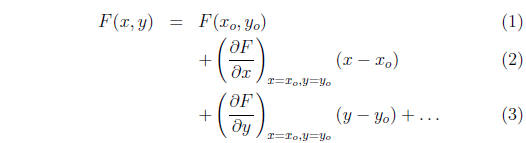
If  is a singular point, the first term is zero . The
terms
is a singular point, the first term is zero . The
terms
represented by . . . are “higher order” and are negligible (if
is small, then  is smaller!). In other words: any smooth
curve under a microscope looks like a straight line!
• Note: Often, you don’t need to compute all those derivatives to
get your Taylor Series. For example, synthetic division is often
an easier way to do things (what is the Taylor series of 1/(1 − x)
about x = 0.2?).
• So, any 2-dimensional singular point under a microscope can be
looked at in the phase plane:

where a, b, c, e are constants and the . . . are terms we
are neglecting
under the microscope. You are expected to be able to fully discuss
a singular point with given values of a, b, c, e, using information
about the eigenvalues and eigenvectors.
• With the . . . terms neglected, you can make statements
about the
stability of the original system using the local linearized analysis.
Your linear conclusions are applicable to the case when the . . .
terms are not summarily neglected EXCEPT for the case of purely
imaginary eigenvalues. You should know why this special case
needs special attention.
• Limit cycles! What is a limit cycle? What are tell tale signs that
there is a limit cycle lurking in your two-dimensional phase plane
sketch?
3. Chapter 6, Laplace Transform. You will be given a xeroxed copy
of the table on page 300.
•You must know the definition of Laplace transform. Even though
the table on page 300 is given to you, I will ask you to work out
some of them long hand.
•You need to refresh your partial fractions. You will need it.
•You need the convolution integral which is item #16 on the table.
•You need to know how to use the step function
 to extract
parts of a given function f (t).
•You need to know the Dirac Delta function
 and how to
compute its Laplace transform.
•You must know how to evaluate the following integral

for t < 17.85 and for t > 17.85.
4. Chapter 5. Series Solutions of Second Order Equations . The
inspired guess is: the solution near the point
 is a power series of
 ! The attention here is limited to linear, second order ODE’s:

Without loss of generality, we set
 .
.
• If P(0) ≠ 0, then x = 0 is an ordinary point. The power
series
is a Taylor series. The only trick you need to practice is how to
shift the index of summation.
• If P(0) = 0, then x = 0 is a singular point. There are two kinds
of singular points: regular and irregular.
• You need to know how to identify a regular singular point (use
the definition given in the book). Once it is identified as a regular
singular point, an inspired guess for the solution is the product of
x r and an innocent ordinary-looking Taylor series. Here r is called
the exponent of the regular singular point. It is determined by the
indicial equation which is a quadratic (for second order ODE’s).
• The mechanics of working such problems is straight forward: use
the trick of shifting the indices of summation to get “all” the
terms under a single summation sign with the same xn factor, any
“left over” terms are then written out explicitly. Setting each of
the leftover terms to zero gives you the “indicial equation,” and
explicit values of some early coefficient. Setting the coefficient of
x n in your big summation term gives you the “recurrence relation.”
Viola, its done.
• If  and
and  is not an integer, then you are in luck.
You need to be able to do such problems, getting two linearly
independent solutions using  and
and
 one after the other.
• If  or
is an integer (both
or
is an integer (both  and
and
 are real), you
need to know there is a problem, and you need to know where to
go in Boyce and Diprima to find the inspired guess for the second
solution.
• We did not cover irregular singular point. If you are confronted
with such a singular point, you are more or less on your own to get
your inspired guess. A good inspired guess is: try an exponential
factor in place of xr and see if it works.
Good luck!
| Prev | Next |