A Unified Framework for Numerical and Combinatorial Computing
A Unified Framework for Numerical and Combinatorial Computing
A rich variety of tools help researchers with
high-performance numerical computing, but
few tools exist for large-scale combinatorial computing. The authors describe
their efforts to
build a common infrastructure for numerical and combinatorial computing by using
parallel
sparse matrices to implement parallel graph algorithms .
Modern scientific applications often
mix combinatorial computing and
numerical computing. Scientists
have found that they can often
gain key scientific insights by studying the relationships
between a system’s individual elements,
rather than studying them in isolation. Combinatorial
data structures such as graphs help describe
such relationships.
Very high-level languages (VHLLs) are already
popular among scientists and engineers. These
languages provide native support for complex
data structures, comprehensive numerical libraries,
and visualization along with an interactive
environment for execution, editing, and debugging.
Matlab and Python are examples of commonly
used VHLLs for scientific computing. In
this article, we focus our attention on Matlab and
Star-P (a parallel implementation of the Matlab
programming language).
Traditionally, numerical algorithms and graph
algorithms have been developed and implemented
separately. Many VHLLs for scientific computing
provide a comprehensive infrastructure for numerical
algorithms, but graph data structures and
algorithms are often deployed as an afterthought,
which restricts their versatility and interoperability
with the rest of the system. Fortunately,
we can unify the diverse worlds of numerical and
combinatorial computing in terms of a common
infrastructure for sparse matrices. Sparse matrices
have long been thought of as graphs, and
many sparse matrix algorithms are built with
graph algorithms.We believe this relationship
can be turned around: graph algorithms can be
efficiently designed and implemented using methods
and systems originally developed for sparse
linear algebra. An early example of this approach
is John R. Gilbert and Shang-Hua Teng’s mesh-
partitioning
toolbox.
Sparse matrix computations allow structured
representation of irregular data structures and access
patterns in parallel applications. In our work,
we use the distributed sparse matrix type in Star-
P as the basis for an infrastructure for computing
with graphs. This approach has many desirable
characteristics: the implementation is written
in the VHLL (here, Matlab), making the codes
short, simple, and readable; the VHLL code is
data-parallel, with a single thread of control. This
makes it easier to write and debug programs, so
the efficiency of the graph algorithms depends
on the efficiency of the underlying sparse matrix
infrastructure’s efficiency. Parallelism is derived
from operations on parallel sparse matrices.
We use the graph primitives described here
to implement several graph algorithms in the
graph algorithms and pattern discovery toolbox
(GAPDT) we developed. From the outset, we
designed the toolbox to run interactively with
terascale graphs via Star-P, scaling to tens or
hundreds of processors. High performance and
interactivity are this toolbox’s salient features.
Sparse Matrices and Graphs
A graph consists of a set V of nodes connected by
directed or undirected edges E. We can specify a
graph with tuples (u, v, w) to indicate a directed
edge of weight w from node u to node v; this is
the same as a nonzero w at location (u, v) in a
sparse matrix. The storage required is θ(|V| +
|E|). A symmetric sparse matrix represents an
undirected graph.
Every sparse matrix problem is a graph problem,
and every graph problem is a sparse matrix
problem. Gilbert, Cleve Moler, and Rob Schreiber
discuss the basic design principles for a comprehensive
sparse matrix infrastructure, and Viral
B. Shah and Gilbert describe additional considerations
for parallel environments. Let’s reiterate
some of the basic design principles for sparse
matrix data structures and algorithms:
•The storage for a sparse matrix of size n-by-n
with nnz nonzeros should be θ(max(n, nnz)).
•An operation on sparse matrices should take
time approximately proportional to the size of
the data accessed and the number of nonzero
arithmetic operations on it.
These principles assure efficient operations on
graphs as well. Consider, for example, constructing
a graph from edge-vertex tuples. The
sparse() function accepts three vectors (U, V,
W) and constructs a sparse matrix G with a nonzero
w at location (u, v) in the sparse matrix. In
our terms, G is also a graph with an edge of weight
w between nodes u and v. We can recover edgevertex
tuples from a graph by using the dual of
sparse(), which is find. Both these operations
take time proportional to the number of nonzeros
in the sparse matrix or the number of edges and
nodes in the graph.
Similarly, we can express many graph queries
as sparse matrix operations. The function
| Table 1. Simple sparse matrix
operations that perform basic graph operations. |
|
| Sparse matrix operation | Graph operation |
| G = sparse (U, V, W) | Construct a graph from an edge list |
| [U, V, W] = find (G) | Obtain the edge list from a graph |
| vtxdeg = sum (spones(G)) | Node degrees for an undirected graph |
| indeg = sum (spones(G)) | In-degrees for a directed graph |
| outdeg = sum (spones(G), 2) |
Out-degrees for a directed graph |
| outdeg = sum (spones(G), 2) |
Out-degrees for a directed graph |
| N = G(i, :) | Find all neighbors of node i |
| Gsub = G(subset, subset) | Extract a subgraph of G |
| G(i, j) = W | Add or modify graph edges |
| G(i, j) = 0 | Delete edges from a graph |
| G(I, :) = [ ] G(:, I) = [ ] |
Delete nodes from a graph |
| G = G(perm, perm) | Permute nodes of a graph |
| reach = G * start | Breadth-first search step |
spones(G) replaces all edge weights with edge
weight 1, which lets us compute in-degrees of
nodes as column sums and out-degrees as row
sums. For undirected graphs, the in-degrees and
out-degrees are the same, but in a sparse matrix,
the row and column sums are equal because such
a matrix is symmetric.
Modern scientific languages derive a great deal
of their expressive power from indexing operations,
and sparse matrix indexing is a powerful
notation for manipulating graphs. The neighbors
of node i in graph G, for example, are the offdiagonal
nonzeros in row i of the sparse matrix
representing G. The indexing operation that performs
this operation is N = G(i, :). We can extract
an induced subgraph of G by selecting the rows
and columns corresponding to the desired nodes
from the corresponding sparse matrix. This looks
like Gsub = G(subset, subset), where subset
is a list of nodes in the resulting subgraph.
Matrix indexing on the right-hand side extracts
submatrices, or subgraphs; matrix indexing on the
left-hand side results in assignment. We can also
relabel graph vertices by permuting the rows and
columns symmetrically. If perm is a permutation
of 1:n, for example, the operation G = G(perm,
perm) relabels the nodes of G according to the
permutation. Table 1 lists these and other corresponding
matrix and graph operations.
GAPDT provides several tools to manipulate
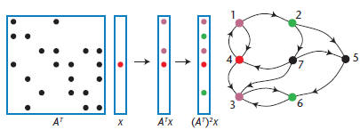
Figure 1. Breadth-first search implemented with sparse
matrix/sparse
vector multiplication. We initialize a sparse vector with a 1 in the
position corresponding to the start node. Repeated multiplication
yields multiple breadth-first steps on the graph. The graph can be
either directed or undirected.
function C = contract (G, labels)
% Contract nodes of a graph
n = length (G);
m = max(labels);
S = sparse (labels, 1:n, 1, m, n);
C = S * G * S’;
Figure 2. Parallel graph contraction. We can
perform this contraction via sparse matrix
multiplication.
graphs, including scalable graph generators for
Erdös-Rényi random graphs, several kinds of
meshes, and power law graphs . It also includes
several graph algorithms, such as breadth-first
search, connected components, strongly connected
components, maximal independent set,
maximum weight-spanning tree, and graph contraction.
The toolbox provides scalable routines for
graph partitioning and clustering and a geometric
mesh-partitioning algorithm for partitioning
large, well-formed meshes. We’ve also included a
spectral graph-partitioning algorithm for general
graphs and non- negative matrix factorization algorithms
for clustering. Because visualization is
an important component of any interactive tool,
we provide a scalable visualization routine to view
the structure of large graphs.
Graph Algorithms
Let’s review our implementation of a few common
graph algorithms to demonstrate the
versatility of the array-based infrastructure:
breadth-first search, connected components, and
graph contraction.
Breadth-First Search
We can perform a breadth-first search by multiplying
a sparse matrix A with a sparse vector x.
Consider such a search starting from node i. We
take x to be a vector with x(i) = 1 and all other
elements zero. The product y = A * x simply picks
out column i of A, which contains the neighbors
of node i. (If the graph is directed, this produces
the in-neighbors of i; to produce the out-neighbors,
we would compute xTA or ATx.) Repeating
the multiplication yields a vector that’s a linear
combination of all columns of A corresponding to
the nonzero elements in vector x, or all nodes that
are—at most—distance 2 from node i. Figure 1
shows a breadth-first search on a directed graph.
We can perform several independent breadthfirst
searches simultaneously by using sparse matrix/
matrix multiplication. Instead of multiplying
with a vector, we multiply with a matrix, with one
column for each starting node. Thus, we compute
Y = A * X, after which column j of Y contains the
result of performing an independent breadth-first
search starting from the node (or nodes) specified
by column j of X. The total work to perform a
breadth-first search with sparse matrix multiplication
is the same as that obtained via other efficient
graph data structures.
Connected Components
A connected component of an undirected graph
is a maximal connected subgraph. Every node
in the graph belongs to exactly one connected
component.
We implement an algorithm from Baruch Awerbuch
and Yossi Shiloach to find connected components
of a graph in parallel.11 The algorithm
works by combining trees of nodes, such that
all nodes in a given tree belong to the same connected
component; the roots of the trees serve as
node labels. The algorithm finishes with one tree
per component, labeling each graph node with the
root of its component’s tree.
We store the trees in a parent vector P; the parent
of node i is stored in P(i). We then use pointer
jumping to find nodes that belong to the same
connected component. Pointer jumping replaces
a node’s label with that of its parent. Repeating
this step several times traverses the trees stored
in P, replacing a node’s label with that of its ancestor.
Eventually, all nodes that belong to the same
component will have the same label as that of the
root of the tree. Because the trees are stored in
a vector, pointer jumping can be performed by
vector indexing—for example, P = P(P) performs
one jump, simultaneously replacing all node labels
with their parent labels. We obtain parallelism
from data-parallel operations on large vectors.8
Graph Contraction
Many graph algorithms proceed by solving the
problem in question iteratively on smaller subgraphs.
But nodes in a graph are sometimes relabeled
during a computation, resulting in nodes
sharing labels. Graph contraction combines nodes
with the same label, merging edges incident on
those nodes as well.
We can efficiently implement contraction in
terms of multiplication via a strategically chosen
sparse matrix. The code fragment in Figure 2
shows how: it creates a sparse matrix S with n nonzeros
(all ones). The column index of each nonzero
is a node’s original label, whereas the row index is
its new label in the contracted graph. As a result,
nodes to be combined end up sharing the same
row in S. Multiplying the graph G with S from
the left combines rows that share labels; similarly,
multiplying G with the transpose of S from the
right combines columns with the same label.
When contraction causes edges to merge, this
implementation adds their weights together. We
can apply different rules for the weight of merged
edges by performing matrix multiplication over
different semi-rings.
Applications
Two applications give a feel for our infrastructure:
the first is a purely combinatorial graph-clustering
benchmark, and the second is an application
in computational ecology that combines numerical
and combinatorial methods to model connectivity
in heterogeneous landscapes.
Graph Clustering
Our implementation of a graph-clustering benchmark
arose from the HPCS Scalable Synthetic
Compact Applications project. The benchmark
consists of multiple kernels that access a single
data structure representing a directed multigraph
with weighted edges. Additional information appears
elsewhere.
The data generator generates an edge list in random
order for a multigraph of sparsely connected
cliques, as Figure 3 shows. The four kernels are
1.Create a data structure for the later kernels.
2.Search the graph for a maximum weight edge.
3.Perform breadth-first searches from a set of
start nodes.
4.Recover the clusters from the undirected
graph.
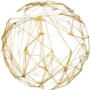
Figure 3. Undirected graph from the graphclustering
benchmark. This visualization is
produced by relaxing the graph’s Fiedler
coordinates projected onto a sphere.
Our implementation of these four kernels is a
couple of hundred lines of code, and it works on
shared as well as distributed-memory architectures
(Star-P runs on both architectures). Kernel
1 uses the sparse() function to create a graph
from an edge list, Kernel 2 uses the find function
to locate the maximum weight edge, and Kernel 3
uses sparse matrix/sparse matrix multiplication for
parallel breadth-first search. For Kernel 4, we experimented
with both breadth-first-search-based
“seed growing” methods and “peer pressure” algorithms6.8
to recover the clusters (see Figure 4).
We ran our implementation of the graph benchmark
in Star-P and used a graph generated with
2 million nodes (scale 21). The multigraph has
321 million directed edges; the undirected graph
corresponding to the multigraph has 89 million
edges. The graph has 32,000 cliques, the largest
with 128 nodes. Because the input graph is a collection
of sparsely connected cliques, most of the
edges are within cliques—in this case, there are
only 212,000 undirected edges between cliques.
All kernels except Kernel 3 scale with the number
of processors, as shown in Figure 5. Kernel 3
doesn’t scale in our implementation (even though
sparse matrix multiplication does scale) because of
the excessive overhead of client-server communication
within Star-P.
Computational Ecology
Circuitscape, a tool written originally in Java
and now in Matlab, uses circuit theory to model
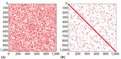
Figure 4. Clusters. (a) A spy plot of the input graph, and
(b) the result
of clustering in Kernel 4. Clusters are revealed as dense blocks on the
diagonal.
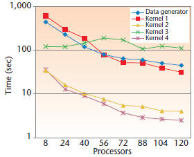
Figure 5. Execution times for the graph benchmark
in Star-P. We generated the input graph with scale
21 and ran the benchmark on an SGI Altix with 128
Itanium II processors and 128-Gbytes of RAM.
animal movement and gene flow in heterogeneous
landscapes. Landscapes are modeled as resistive
networks; current flow across a model landscape
takes into account multiple dispersal pathways,
which can be useful in explaining patterns of gene
flow and genetic differentiation among animal
populations.
Analyzing a landscape requires first converting
the landscape of interest into a graph, with areas
between whose connectivity is to be measured
(such as nature reserves or animal populations)
represented as polygons. To accomplish this, Circuitscape
first reads a raster cell map as an m × n
conductance matrix, where each nonzero element
represents a cell in the landscape. Next, it uses
stencil operations to convert the m × n conductance
matrix into a graph with mn nodes. Graph
edges correspond to connections between cells
in the landscape, typically first- or second-order
neighbors. Habitats, which span several cells, are
contracted into a single graph node. As a result, all
cells neighboring a habitat become neighbors of
the contracted node. The connected components
algorithm then removes any disconnected parts
of the landscape. Finally, Circuitscape constructs
the graph Laplacian with elementary matrix operations
and uses Kirchoff’s laws to compute current
flows by solving a sparse linear system.
These operations use both combinatorial and
numerical algorithms. Combinatorial algorithms
first preprocess the landscape graph (see Figure
6a), so that numerical algorithms can then compute
current flows in the landscape (see Figure
6b). Even at moderate resolutions, the underlying
graphs of habitat maps can be quite large,
depending on the size of the landscape and the
species being modeled. At large scales, combinatorial
algorithms are also used to compute a preconditioner15
to accelerate the iterative solution
of linear systems.
The original Circuitscape code ran sequentially
and typically took several hours to process
a landscape with hundreds of thousands of cells; a
landscape with a million cells took roughly three
days. Our improvements included using GAPDT
to speed up the combinatorial computations and
iterative methods to speed up the solutions of
linear systems (and allow memory use to scale),
introducing parallel processing with Star-P, and
general vectorization. The new Circuitscape can
process landscapes with as many as 40 million
cells in an hour.
Although high-performance numerical
computing is a well-developed field,
high-performance combinatorial computing
is in its infancy. Our work aims
to build on the large body of tools and techniques
for numerical computing (in particular, for sparse
matrix computation) to create efficient, effective,
usable tools for large-scale problems that require
both discrete and numerical computation.
In ongoing work, we’re extending our sparse
matrix infrastructure to accommodate a larger
variety of graph algorithms. One example is supporting
sparse matrix multiplication on arbitrary
semi-rings: graph construction from triples currently
only lets us add duplicate edges, and we’d
like to allow other user-defined schemes. Another
exciting research problem is the choice of sparse
structures and algorithms to efficiently manipulate
“hypersparse” graphs, which arise in highly
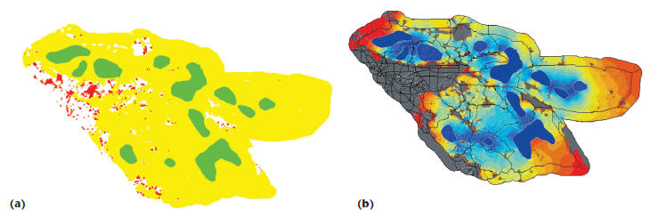
Figure 6. Connectivity modeling for mountain lions in
Southern California. In (a), disconnected parts of the landscape are
shown in red, and habitats, which are contracted nodes, are shown in green. The
result of the combinatorial phase is used as
an input to the numerical phase (b), which shows current flow across the
landscape
parallel settings. General submatrix indexing and
sparse matrix/matrix multiplication are examples
of primitives that are ubiquitous in array-based
sparse graph algorithms but haven’t been studied
extensively by the numerical computing community;
developing more efficient algorithms (which
could be polyalgorithms) for such primitives is a
fertile area for further research.
| Prev | Next |