Systems of Linear Equations

Given a system of equations

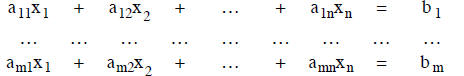
we wish to find all solutions. The equations are said to be inhomogeneous since the constants on the
right hand side are not 0. Associated with this system is a homogeneous system ( called the reduced
homogeneous system of the original system) given by

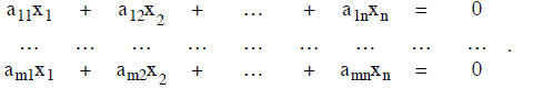
In matrix notion the inhomogeneous and the homogeneous systems are represented by Ax = b and
Ax = 0 respectively.

We note that set of solutions of the homogeneous system has a special form.

THEOREM. The set of solutions of the homogeneous system of equations Ax = 0 is a subspace of

REMARK. The set of solutions of Ax = 0 is called the null space of A or the kernel of A and is
denoted by Null A or ker A

PROOF. If y and z are in K = Null A, we must show that ay + bz is also in K in order to show that K
is a subspace of . We just test this out by the defining property of K , viz., that A annihilates each
vector of K. Here, to test this out we use some properties of matrix multiplication . We have that

A(ay + bz) = aA(y) + bA(z) = a0 + b0 = 0.

So ay + bz is in K and thus K is a subspace. Q.E.D.

The theorem governing the relation of an inhomogeneous system and its associated homogeneous
systems is the following:

THEOREM. Let Ax = b be a system of equations. Let S be the set of all solutions of the reduced
homogeneous system Ax = 0. Let x_p be one particular solution of the original system Ax = b. Then

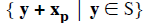
is the set of all solutions of the system Ax = b.
PROOF. First let y ∈S. Then we have that y + x_p is a solution of Ax = b since

Now let z be a solution of Ax = b. Then we have that

So we have that y = z - x_p is a solution of Ax = 0 and thus y ∈S. This means that z has the desired
form z = y + x_p. Q.E.D.

If we can find the one particular solution x_p of Ax = b by some method even by guessing, we
would just have to produce all solutions of the associated homogeneous system Ax = 0 and add x _p to
all solutions of Ax = 0 to find all solutions Ax = b. This is the content of the preceding theorem.
However, our method of Gaussian elimination to upper triangular form from which the solutions are
read off produces all solutions of the inhomogeneous system at one stroke

EXAMPLE. Solve for all solutions the system of equations

SOLUTION. We write down the Gaussian steps for the augmented matrix as

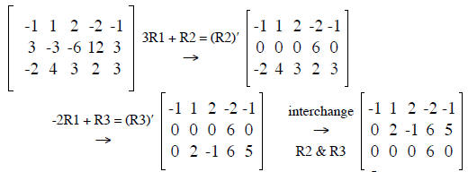
We read of the solution x₄ = 0, x₃ = s (a variable),.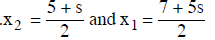

We write this in vector form as

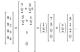
Since we are interested in the last expression for all , we may replace s/2 by t to get

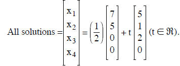
We see that

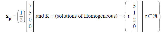
Instead of using a variable , we can generate a basis of the null space numerically. Suppose that
the coefficient matrix A of the homogeneous system is taken to row reduced form B. Suppose the
columns j₁, … , j_p are non pivot colunms. These columns take a variable in our method of solution.
Instead of using a variable, we substitute alternately a single 1 and p - 1 0’s for the coordinates, i.e., we
substitute (1, 0, 0, … , 0), (0, 1, 0, … , 0), (0, 0, 1, … , 0), … , (0, 0, 0, … , 1) in the columns j₁, … , j_p
and read off the rest of the n - p coordinates for the pivot columns. We get p vectors which will be a
basis for the kernel K. For example in our case, we use Gaussian elimination to get

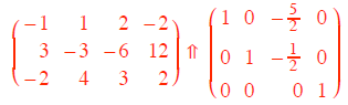
We then set the single nonpivot element x₃ = 1 and read of the solutions as x₄ = 0, x₃ = 1/2 and x₁ =
5/2. So the vector v = (5/2, 1/2, 1, 0) is a basis of the Null Space of A.

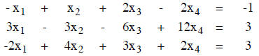
EXAMPLE. Consider the system of equations

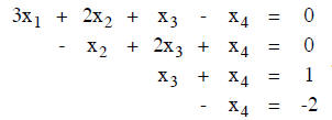
The augmented matrix is

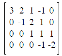
and the solution can be read off as x₄ = 2, x₃ = 1 - x₄ = -1, x₂ = 2x₃ + x₄ = 0, and
x₁ = (1/3)(x₄ - x₃ - 2x₂) = 1. Here

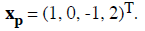
The solution space of the associated homogeneous system is K = {0}, and thus, the associated
homogeneous system only has the trivial solution 0. In general, when only the solution x_p is showing
in the solution, the solution of the associated homogeneous solution is only the trivial solution.