Linear Algebra
If you are unfamiliar with linear or matrix algebra, you
will find that it is
very different from basic algebra or calculus . For the duration of this session,
we will be focusing on definitions of such concepts as linear equations,
matrices,
determinants, vector spaces, inner products , linear transformations, eigenvalues
and eigenvectors, and their applications to interesting mathematical problems.
Texts:
Linear Algebra and Its Applications (3rd Edition) Addison
Wesley © 2003,
by David C. Lay (DCL)
Module 1
Properties of Matrices
System of Linear Equation
DCL (Recommended):
1.1.16, 22, 30
1.6.8, 14, 15
1.7.1, 3, 5, 11
1.8.1, 3, 15, 21
Module 2
Linear Independence
Inverse of Matrix Linear Systems and Inverses
Determinants
DCL(Recommended):
2.1.3, 5, 7, 10, 15, 16, 19, 25
3.1.1, 9, 11, 19, 21
3.2.3, 9, 10
Module 3
Eigenvalues/Eigenvectors
Cramer's Rule
Orthogonality(?)
DCL(Recommended):
5.1.3, 4, 5, 7, 8
5.2.7, 9
5.3.3, 11, 13
6.1.3, 5, 7
6.2.5, 7
6.3.3, 9, 11
1 Linear Algebra: Module
1.1 Module Topics:1
System of Linear Equations
Method of Substitution
Gaussian Elimination
Gauss-Jordan Elimination
Matrix Methods
1.1.1 Linear Equation
a1x1 + a2x2 + … + anxn = b
4x1 - 5x2 + 2 = x1 → rearranged →
x2 = 2( - x1) + x3 → rearranged →
1.1.2 Systems of Linear Equations
Collection of one or more linear equations involving
Collection of one or more
linear equations involving same variables say x1,…, xn. An example is
x1 - 2x2 + x3 = 0
2x2 - 8x3 = 8
-4x1 + 5x2 + 9x3 = -9
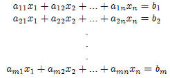
More generally, we might have a system of m equations in n unknowns
The set of all possible solutions is called the solution
set of the linear system.
Two linear systems are called equivalent if they have the same solution sets.
Finding the solution set of a system of two linear equations in two variables
is easy because it amounts to finding the intersection of two lines.
| x1 + x2 = 10 -x1 + x2 = 0 |
x1 - 2x2 = -3 2x1 - 4x2 = 8 |
x1 + x2 = 3 - 2x1 - 2x2 = -6 |
If there are three equations in three variables, each
equation would define a
plane in a 3 dimensional space. Same reasoning applies. If there are more than
3 variables, the intersection of hyperplanes would determine the solution set.
1.1.3 Strategies for Solving a System
In order to solve the system of linear equations, we can
utilize all or one of the
following three strategies:
1. Substitution
2. Elimination (of variables)
3. Matrix Methods
Method of Substitution Steps:
1. Solve one equation for one variable, say x1, in terms of the other
variables in the equation
2. Substitute the expression for x1 into the other m-1equations, result-
ing in a new system of m - 1 equations in n - 1unknowns.
3. Repeat steps 1 & 2 until one equation in one unknown, say xn. We
now have a value for x n.
4. Backward substitution: substitute xn into previous equation(s). Re-
peat using the successive expressions of each variable in terms of the other
variables to …nd the values of all

Using substitution, solve:
x1 - 2x2 = -1
-x1 + 3x2 = 3
Using substitution, solve:
x1 - 2x2 + x3 = 0
2x2 - 8x3 = 8
-4x1 + 5x2 + 9x3 = -9
Method of Elimination a) Elementary Row Operations
Elementary row operations are used to transform the equations of a linear
system, while maintaining an equivalent linear system - equivalent in the sense
that the same values of xj solve both the original and transformed systems.
These operations are
1. (Replacement) Add one row to a multiple of another row.
2. (Interchange) Interchange two rows.
3. (Scaling) Multiply all entries in a row by a nonzero constant.
Take Example 2, for instance, we can:
Add the 1st row to the 2nd row of equation to get:
x1 - 2x2 = -1
x2 = 2
Then use backward substitution to get
x1 = 3
x2 = 2
We can apply the similar procedure to solve for Example 3
x1 - 2x2 + x3 = 0
2x2 - 8x3 = 8
-4x1 + 5x2 + 9x3 = -9
(i) To do so, add 4 times 1st row to the 3rd row of equation. To get a
new 3rd row of equation.
(ii) Now, multiply equation 2 by 1/2 in order to obtain 1 as the coefficient
for x2. (This calculation will simplify the arithmetic for the next step.)
(iii) Use the x2 in equation 2 to eliminate the -3x2 in equation 3 in
order to obtain:
(iv) The new system has a triangular form:
We can use backward substitution to fi…nd the solution set.
Check to see if (29, 16, 3) is a solution of the original system.
b) Gaussian Elimination
Method by which we start with some linear system of m equations in n
unknowns and use the elementary equation operations to eliminate variables
until we arrive at an equivalent system of the form:
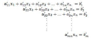
The bold faced coe¢ cients are referred to as pivots.
(Essentially similar to the method shown above)
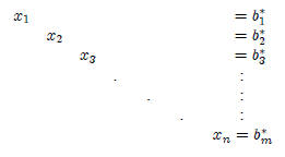
c) Gauss-Jordan Elimination
Takes the Gaussian elimination method one step further . Once the linear
system is in the reduced form shown in the preceding section , elementary row
operations and Gaussian eliminations are used to
(i) Change the coefficient of the pivot term in each equation to 1
and
(ii) Eliminate all terms above each pivot in its column,
resulting in a reduced, equivalent system. For a system of m equations in n
unknowns, a typical reduced system would be:
d) Matrix Method
Matrices provide an easy and efficient way to represent linear systems such
as:
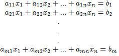
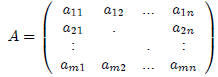
The m × n coefficient matrix A is an array of mn real numbers arranged
in m rows by n columns.
The RHS of the linear system is represented by the vector

Augmented matrix: when we append b to the coefficient matrix A, we get
the augmented matrix
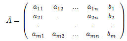
The rules of elementary row operations apply here.
Gaussian elimination of the augmented matrix results in a row echelon
form.
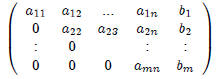
Note:
(i) All nonzero rows are above any rows of all zeros.
(ii) Each leading entry of a row is in a column to the right of the
leading entry of the row above it.
(iii) All entries in a column below a leading entry are zeros.
Reduced row echelon form
Satisfies the following additional conditions
(iv) The leading entry in each nonzero row is 1.
(v) Each leading 1 is the only nonzero entry in its column.
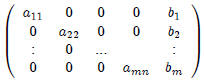
In essence, this is the matrix equivalent of a linear system after Gauss-Jordan
elimination.
| Prev | Next |