INTRODUCTION TO MATLAB
Chapter 4
Arrays and x-y Plotting
4.1 Colon (:) Command
Simple plots of y vs. x are done with Matlab's plot command and arrays.
These arrays
are easily built with the colon (:) command. To build an array x of x- values
starting at
x = 0, ending at x = 10, and having a step size of h = .01 type this:
clear,close all, % close the figure windows
x=0:.01:10,
Note that the semicolon at the end of this line is
crucial , unless you want to see 1001
numbers scroll down your screen. If you do make this mistake and the screen
print is going
to take forever, ctrl-c will rescue you.
An array like this that starts at the beginning of an
interval and finishes at the end of
it is called a cell-edge grid. A cell-center grid is one that has N
subintervals, but the data
points are at the centers of the intervals, like this
dx=.01,
x=.5*dx:dx:10-0.5*dx,
Both kinds of grids are used in computational physics.
(Note: Matlab's linspace command
also makes cell-edge grids. Check it out with help linspace.)
And if you leave the middle number out of this colon
construction, like this
t=0:20,
then Matlab assumes a step size of 1. You should use the
colon command whenever possible
because it is a pre-compiled Matlab command. Tests show that using : is about 20
times
faster than using a loop that you write yourself (discussed in Chapter 9). To
make a
corresponding array of y values according to the function y(x) = sin(5x) simply
type this
y=sin(5*x),
Both of these arrays are the same length, as you can check
with the length command (Note
that commands separated with commas just execute one after the other, like
this:)
length(x),length(y)
4.2 xy Plots, Labels, and Titles
To plot y vs. x, just type this
close all, % (don't clear--you will lose the data you want to plot)
plot(x,y,'r-'),
The 'r-' option string tells the plot command to plot the
curve in red connecting the dots
with a continuous line. Other colors are also possible, and instead of
connecting the dots
you can plot symbols at the points with various line styles between the points.
To see what
the possibilities are type help plot.
And what if you want to plot either the first or second
half of the x and y arrays? The
colon and end commands can help:
nhalf=ceil(length(x)/2),
plot(x(1:nhalf),y(1:nhalf),'b-')
plot(x(nhalf:end),y(nhalf:end),'b-')
To label the x and y axes, do this after the plot command:
xlabel('\theta')
ylabel('F(\theta)')
(Note that Greek letters and other symbols are available
through LaTex format-see Greek
Letters, Subscripts, and Superscripts in Section 4.8.) And to put a title on you
can do this:
title('F(\theta)=sin(5 \theta)')
You can even build labels and titles that contain numbers
you have generated, use Matlab's
sprintf command, which works just like fprintf except that it writes into a
string
variable instead of to the screen. You can then use this string variable as the
argument of
the commands xlabel, ylabel, and title, like this:
s=sprintf('F(\\theta)=sin(%i \\theta)',5)
title(s)
Note that to force LaTex symbols to come through correctly
when using sprintf you have
to use two backslashes instead of one.
4.3 Generating Multiple Plots
You may want to put one graph in figure window 1, a second plot in figure
window 2, etc.
To do so, put the Matlab command figure before each plot command, like this
x=0:.01:20,
f1=sin(x),
f2=cos(x)./(1+x.^2),
figure
plot(x,f1)
figure
plot(x,f2)
And once you have generated multiple plots, you can bring
each to the foreground on your
screen either by clicking on them and moving them around, or by using the
command
figure(1) to pull up figure 1, figure(2) to pull up figure 2, etc. This might be
a useful
thing to use in a script. See online help for more details.
4.4 Overlaying Plots
Often you will want to overlay two plots on the same set of axes. There are
two ways you
can do this.
| Example 4.4a (ch4ex4a.m)
% Example 4.4a (Physics 330)
%********************************************************* % plot both plot(x,y,'r-',x,y2,'b-')
%********************************************************* figure |
You can now call as many plots as you want and they will
all go on the same gure. To
release it use the command
hold off
as shown in the example above.
4.5 xyz Plots: Curves in 3-D Space
Matlab will draw three-dimensional curves in space with the plot3 command.
Here is how
you would do a spiral on the surface of a sphere using spherical coordinates.
| Example 4.5a (ch4ex5a.m) % Example 4.5a (Physics 330) clear, close all, dphi=pi/100, % set the spacing in azimuthal angle N=30, % set the number of azimuthal trips theta=phi/N/2, % go from north to south once r=1, % sphere of radius 1 % convert spherical to Cartesian % plot the spiral |
4.6 Logarithmic Plots
To make log and semi-log plots use the commands semilogx, semilogy, and
loglog. They
work like this.
| Example 4.6a (ch4ex6a.m) % Example 4.6a (Physics 330) clear, close all, x=0:.1:8, semilogx(x,y), figure figure |
4.7 Controlling the Axes
You have probably noticed that Matlab chooses the axes to t the functions
that you are
plotting. You can override this choice by specifying your own axes, like this.
close all,
x=.01:.01:20,
y=cos(x)./x,
plot(x,y)
axis([0 25 -5 5])
Or, if you want to specify just the x-range or the
y-range, you can use xlim:
plot(x,y)
xlim([ 0 25])
or ylim:
plot(x,y)
ylim([-5 5])
And if you want equally scaled axes, so that plots of
circles are perfectly round instead
of elliptical, use
axis equal
4.8 Greek Letters, Subscripts, and Superscripts
When you put labels and titles on your plots you can print Greek letters,
subscripts, and
superscripts by using the LaTex syntax. (See a book on LaTex for details.) To
print Greek
letters just type their names preceded by a backslash , like this:
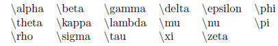
You can also print capital Greek letters, like this
\Gamma, i.e., you just capitalize the first
letter.
To put a subscript on a character use the underscore
character on the keyboard:  is
is
coded by typing \theta 1. And if the subscript is more than one character
long do this:
\theta {12} (makes  ). Superscripts work the
same way only using the ^ character: use
). Superscripts work the
same way only using the ^ character: use
\theta^{10} to print 
To write on your plot, you can use Matlab's text command
in the format:
text(10,.5,'Hi'),
which will place the text "Hi" at position x = 10 and y = 0:5 on your plot.
You can use LaTex Greek in labels and titles too. If you
want Matlab to layout an
equation like LaTex would (rather than just getting the Greek letters in your
labels), you
use the following syntax:
title('Plot of $\frac{\sin(x)}{x}$','Interpreter','Latex')
With this interpreter, you type text and equations in
regular LaTex syntax and Matlab
will use LaTex to typeset the text. (Read a LaTex tutorial for further
information on this
format.)
4.9 Changing Line Widths, Fonts, Etc.
You can also use a number of graphical tools to change line widths, put text
and lines on
the plot, etc. To do this, click the "Show Plot Tools" button on the toolbar. If
you want
to change the look of anything on your plot, like the font style or size of
text, the width of
the lines, the font style and size of the axis labels, etc., just left click on
the thing you want
to change until it is highlighted, then right click on it and select Properties .
This will take care of simple plots, but if you want to
make publication quality figures
you will have to work harder. See Chapter 17 at the end of this booklet titled
Plots for
Publication for more information.
| Prev | Next |