Solvers of a System of Linear Equations

If we examine the algorithm of the Gaussian elimination, we can easily find that the zeros
outside the band will neither make any affect to the coefficient matrix nor be changed by the
algorithm. That is, we need not store them and we need not process them. This way we can
save the storage space for the coefficient matrix and also we can save computing time by
neglecting them. This is the idea of the band method. Most of systems of linear equations
obtained in the finite element method for linear elastic structure are this type.

As a variation of the Gaussian elimination algorithm , we can find the Crout method that
makes a LU decomposition of the coefficient matrix A by a lower triangular matrix L and
the upper triangular matrix U, or the Cholesski method that makes a LDU decomposition
of A into a lower triangular matrix L, diagonal matrix D, and upper triangular matrix U.
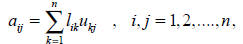
Suppose that a given matrix A is decomposed into a LU form :

LUx = b

where

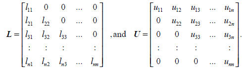
Then the original problem can be decomposed to two matrix equations :

Ly = b and Ux = y

which can be solved easily by the following algorithm :

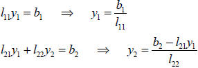
that is

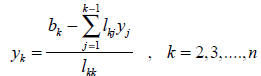
and similarly the second equation can solved as

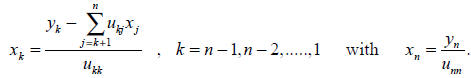
Thus the main issue is how to make a LU decomposition. Noting that

For the first column vector, we have

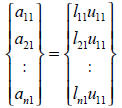
and then if we set up u₁₁ = 1, we can determine the first column of L. Similarly, the first
row becomes

and then we can determine the first row of U. For the second column and row, we have

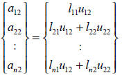
and

By setting u₂₂ = 1, we can determine the second column of L and second row of U.
Continuing this process step by step , yields the LU decomposition. If we examine this
procedure, it can be found that zeros outside the profile limit ( that is called the skyline)
shown in the figure, would not make any contribution to the Crout algorithm, that is, they
need not be stored and can be skipped for their operation .

This method has more advantage than the band method, since we need not keep some of
zeros within the band of the coefficient matrix. Based on this algorithm, many skyline ( or
profile ) methods have been developed for finite element analysis.

Both the band and skyline methods require to form the global stiffness matrix of the whole
structure by assembling all of element stiffness matrices, and then after forming the
coefficient matrix completely, the Gaussian elimination algorithm is applied. Therefore, we
cannot reduce storage space too much because of the size of the global stiffness matrix
which is roughly speaking, mn, where m is the band width and n is the size of the stiffness
matrix, respectively. The wave front method is the one which utilizes the special structure
of the finite element approximation, and is the one which may not require complete
formation of the global stiffness matrix ( that is, the coefficient matrix ). It eliminates the
terms ( components of the coefficient matrix ) whenever they can be eliminated before
assembling the rest of finite element stiffness matrices, but at the moment they are
assembled. In other words, it eliminates the terms “detached” from the rest of the structure
while assembling. For example, node 1 is only used by element <1>, and then the terms
related to node 1 can be eliminated at the time of “assembling” of element <1>, since the
components of the global stiffness matrix related to node 1 are the same with the completely
assembled global stiffness matrix. Similarly, node 2 is sheared with element 1 and element
2, and then at the stage of assembling the element stiffness matrices up to element 2, the
terms related to node can be eliminated. Repeating this elimination procedure while
assembling, the front line of the elimination is moving like waves . It seems that the naming
of the wave front, or frontal method reflects this nature. Since we do not form the global
stiffness matrix in complete form before the Gaussian elimination procedure, it does not
require the space for the global stiffness matrix. It only requires the sufficiently large space
that can store the assembled stiffness matrix related to the elements on the wave front.
Using this nature of the method, Iron could solve fairly large scale problems with relatively
small core memory in computers. At the time Iron introduced his beautiful engineering idea
to solve a system of linear equations , the success of the finite element method became quite
sound. It is strongly recommended that Iron’s monumental work should be thoroughly
studied to understand the role of the finite element method in computer technology.

Iteration Methods

Another way to eliminate the completely assembled global stiffness matrix to reduce the
core memory and storage disk space, is application of iteration methods which requires
only multiplication of the element stiffness matrices and the associated degrees of freedom.
Noting that the global stiffness matrix is formed by assembling of the element stiffness
matrices, we have the following relation

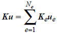
where K is the global stiffness matrix, u is the global generalized displacement vector, K_e
is the element stiffness matrix, u_e is the element generalized displacement vector, and N_e
is the total number of elements . If a system of linear equations

Ku = f

is considered, it is equivalent to the following :

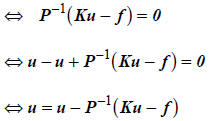
where P is an arbitrary invertible matrix, and is called the pre-conditioning matrix. Using
this relation, we can expect the iteration scheme

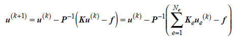
for an initial guess u⁽⁰⁾ . If this algorithm can lead convergence by iteration, we can find the
solution of the system of linear equations. It is clear that this does not require the formation
of the global stiffness matrix. Because of this nature, required core memory can be very
small, and then it was very popular in the early 1960s. However, since it is iterated, its
convergence was not necessarily guaranteed. Furthermore, estimation of the required
iteration number was difficult. Because of such uncertainties in iteration methods, they are
gradually replaced by the direct methods, especially by the wave front method in the finite
element community in the 1970s.

They were, however, revived at the time of introduction of supercomputers in the 1980s
which are specially design with vector and parallel processing. In order to take advantage
of these specially designed computer architecture, we once again found that the iteration
method is the best fit to these new type of computers, and computer scientists started
showing capability to solve more than a million equations. At this moment, the most
promising iteration method is regarded as the preconditioned conjugate gradient method (
PCG method ), convergence of which can theoretically be proven, and required number of
iterations can also be reduced significantly by introduction of an appropriate preconditioning
matrix. It is believed that the iteration method would be dominant for solving
large scale problems involving more that a million equations. At this moment ( 1996 ),
researchers are challenging to solve 10 to 20 million equations.

Figure X Application of a PCG method to FEA by S. Holister ( Voxelcon Inc. ) using
about 150,000 Solid Elements ( Approximately 450,000 degrees of freedom )