Newton Raphson Algorithm
Let f(x) be a function (possibly multivariate) and suppose
we are interested in determining
the maximum of f and, often more importantly, the value of x which maximizes f.
The most
common statistical application of this problem is finding a Maximum Likelihood
Estimate (MLE).
This document discusses the Newton Raphson method
1 Motivation
Newton Raphson maximization is based on a Taylor series expansion of the
function f(x). Specifically,
if we expand f (x) about a point a,

where f'(·) is the gradient vector and f''(·) is the
hessian matrix of second derivatives. This creates
a quadratic approximation for f. We know how to maximize a quadratic function
(take derivatives,
set equal to zero , and solve)
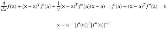
The Newton Raphson process iterates this equation.
Specifically, let  be a starting point for
the algorithm and define successive estimates  recursively through the equation

If the function f(x) is quadratic , then of course the
quadratic “approximation” is exact and the
Newton Raphson method converges to the maximum in one iteration. If the function
is concave,
then the Newton Raphson method is gauranteed to converge to the correct answer.
If the function
is convex for some values of x , then the algorithm may or may not converge. The
NR algorithm may
converge to a local maximum and not the global maximum, it might converge to a
local minimum,
or it might cycle between two points . Starting the algorithm near the global
maximum is the best
practical method for helping convergence to the global maximum.
Fortunately, loglikelihoods are typically approximately quadratic (the reason
asymptotically
normality occurs for many random variables ). Thus, the NR algorithm is an
obvious choice for
finding MLEs. The starting value for the algorithm is often a “ simpler ” estimate
(in terms of ease
of computation) of the parameter, such as a method of moments estimator.
Example
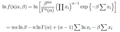
Let  and suppose we want the joint maximum
likelihood estimate
and suppose we want the joint maximum
likelihood estimate
of  . The loglikelihood is
Solving for the MLE analytically requires solving the equations
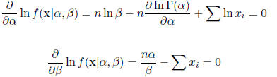
These two equations cannot be solved analytically (the
Gamma function is difficult to work with).
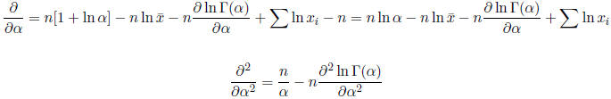
The two equations do provide us with the gradient
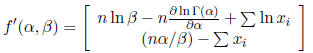
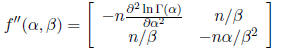
The hessian matrix is
The starting values of the algorithm may be found using
the method of moments. Since 
 and
and 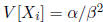 , the
method of moment estimators are
, the
method of moment estimators are  and
and
 .
.
Suppose we have data (in truth actually generated with α = 2 and β =
3) such that n = 1000,
 , and s2 = 0.2235679. The algorithm begins at

2.073976 and  = 3.04577. After 3 iterations,
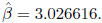
the NR algorithm stabilizes at
= 3.04577. After 3 iterations,
the NR algorithm stabilizes at 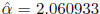 and
and
Note that there is no need to treat this situation as a multivariate problem.
The partial
derivative for β may be solved in terms of α.
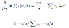
Thus, for each value of α, the maximum of β is
attained at  . Thus, we can reduce the
problem to the one-dimensional problem of maximizing
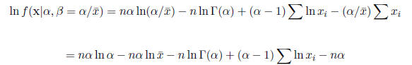
This is called the profile loglikelihood. The first and second derivatives are
Again starting the algorithm at
![]() 2.073976, the
algorithm converges to
2.073976, the
algorithm converges to
![]() after
after
???? iterations.
| Prev | Next |