College Algebra Supplemental Materials

Section: Graphs of Rational Functions

Lesson 1: Rational function Review

This is a review of some things we did in Part II. The main thing to remember is that when
you want to simplify a fraction containing algebra, you want to factor the top and bottom,
then simplify. Remember, the only time you can cancel things in a fraction is when you
are multiplying and dividing by the same thing. We can cancel because multiplication and
division are inverses. That is why you factor, to write the numerator and denominator as
multiplication expressions so you can see what you can cancel. After you’ve done these a
while, you figure out how to do it without actually showing the factoring, but you’re still
doing the same thing. Remember, division and multiplication are inverses, so they cancel.
Division and addition are not inverses, so they don’t cancel.

Lesson 2: Asymptotes of rational functions (Lesson Notes)

Lesson 2: Asymptotes of rational functions

This lesson primarily focuses on the graph of f(x) =1/x. This graph looks like this .

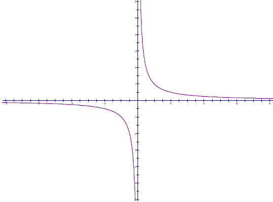
There are a couple of important things to notice about this graph.

• It has a horizontal asymptote of y = 0. That is, as the x-values get really big, the
graph gets closer and closer to the line y = 0 (which is the x-axis). This happens
because when you divide a normal size number by a really big number, you get a
really small number. The same thing happens when the x-values get very negative,
that is to say they move in the direction of positive infinity . The language to describe
this is getting awkward at this point, we’ll talk about this in a minute.

• This graph has a vertical asymptote of x = 0. This is because as the x-values get
closer to zero, we are dividing by a really tiny number, and when you divide a normal
sized number by a really tiny number, you get a really big number. If you don’t
believe me, try dividing 1 (or 2, or 5, or 126) by .0000001 and see what you get.

• This graph is not continuous. That is to say that it has two pieces and it is impossible
to get from the piece to the left of the y-axis to the piece to the right of the y-axis
without leaving the graph, lifting up your pencil, something like that. This is
important because it means that this graph can go from being less than zero to being
greater than zero without ever actually being zero. Very tricky, huh?

There is a word for what we are talking about here when we ask questions such as "What
happens to f(x) as x gets really big?" or "What happens to f(x) as x gets really negative?"
This is called the end behavior of the function. If you think about it, this makes sense.
We are talking about how the function behaves out at the ends of the number line.

Lesson 3: More vertical asymptotes (Lesson Notes)

Because phrases such as "as x gets really big" and "as x gets really negative" don’t
sound like precise mathematical language , we have other ways to say this. Instead of "as x
gets really big," we say "as x goes to positive infinity," which we can write more concisely as
"as x→∞ ." Instead of "as x gets really negative," we say "as x goes to negative infinity,"
which we can write as "as x →∞ ." Similarly, we can talk about what happens to the
function values by writing things like y→∞ ("y goes to infinity") or y→ 0 ("y goes to
zero").

Often, when we talk about x getting close to zero, we need to know if it is coming from
the left or from the right (coming from the negative numbers or from the positive numbers).
When we talk about f(x) =1/x, we need to make this distinction. There is notation for this,
which you will learn if you take calculus, but for now we’re learning enough new notation,
so if we want to talk about x getting close to zero from the left, we’ll just write, "as x →0
from the left."

So we can summarize the behavior of f(x) =1/x like this, (these are important; make
sure they make sense to you.)

• As x→∞ , y →0.
• As x →∞ , y →0
• As x →0 from the left, y→ -∞
• As x →0 from the right, y →∞

In the rest of this lesson, we noticed that all of the things we learned about transformations
of quadratics and other functions will apply to functions like this as well. So the
graph of will look just like the graph of y =1/x except that it is shifted 7 units
to the right and 3 units up.

Lesson 3: More vertical asymptotes

If we have a rational function–that is, a fraction with a polynomial (or a constant) in the
numerator and denominator–then we will have a vertical asymptote for any x-value that
meets two conditions:

• It makes the denominator equal to zero

• It does not make the numerator equal to zero.

If the denominator and the numerator are both equal to zero for a given x-value, then
we will usually have a line or curve with a hole in it. In more technical terms, we say that
the graph has a discontinuity at that particular x-value. It is important to realize that these
discontinuities (holes) won’t show up on your calculator, you have to know they’re there by
paying attention to the domain of the function. (This is one of the reasons we have been
talking about domain so much.)

Lesson 4: More horizontal asymptotes (Lesson Notes)

• Remember: A vertical asymptote is a line and it needs to be written as an equation.
A vertical line has an equation of the form, x = a, where a is a value that you will
have to determine

Lesson 4: More horizontal asymptotes

Note: We are talking about rational functions here. That’s one polynomial divided
by another polynomial, something like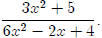If we start adding or subtracting
constants, like we did in lesson 2, then this moves things around.

Horizontal asymptotes are a little bit trickier to figure out. Horizontal asymptotes
happen whenever the function values get closer and closer to a given number as x→∞ .
You can find the horizontal asymptotes of a rational function using the following rules.

• If the degree of the denominator is greater than the degree of the numerator, the
function will have a horizontal asymptote of y = 0.

• If the degree of the numerator is greater than the degree of the denominator, the
function will not have a horizontal asymptote. It may have a slant asymptote, which
we’ll talk about later.

• If the degree of the denominator is the same as the degree of the numerator, the yvalue
of the horizontal asymptote is equal to the quotient of the leading coefficients.
For example, let’s look at the following function.

This will have a horizontal asymptote at y = 4 because12/3= 4.

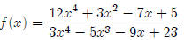
Why is this true? There are a couple of ways to think about this. One way is to
remember that when we are talking about a horizontal asymptote, we are thinking about
what happens when x gets very big (what happens as x→∞ ). As x get very large, the
highest degree terms will get much larger than the lower degree terms. If you think about
it for a minute. If x = 1, 000, then x⁴ is a thousand times bigger than x³. If x = 1, 000, 000,
then x⁴ is a million times bigger than x³.

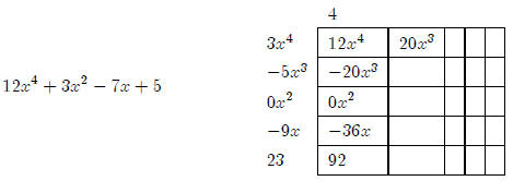
Another way to think about this is to think about the fraction as a division. Let’s look
what happens if we divide12x⁴ + 3x² − 7x + 5 ÷ 3x⁴ − 5x³ − 9x + 23 using rectangle
division. We’ll start in the usual way, by putting the first term in the upper left hand box,

Lesson 4: More horizontal asymptotes (Lesson Notes)

dividing, and then multiplying down.

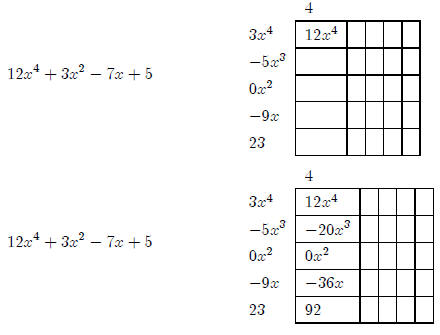
Now we’ll complete the x³ diagonal.

Now we’re stuck. There is nothing we can multiply by 3x⁴ to get 20x³ (we do not want
to get into negative exponents or anything like that). So we’re done. Everything else is a
remainder. So we need to complete the diagonals as much as we can to find our remainder.

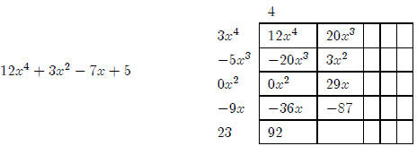
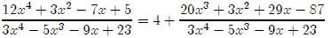
So we have12x⁴ + 3x² − 7x + 5÷3x⁴ − 5x³ − 9x + 23= 4,R (20x³+3x²+29x−87).
That’s right, the answer is 4 with a remainder of (20x³+3x²+29x−87). In other words,

Lesson 5: Logs to different bases (Lesson Notes)

Now, as x gets very large,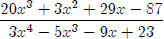is going to get very close to zero, until,
if x is large enough, it doesn’t really matter and the function value will be as close to 4 as
we want it to be.

This all looks very complicated and it might seem like nuisance to find these long
complicated remainders, because it is a nuisance. But we don’t have to find the remainder,
the point here is that when we are talking about horizontal asymptotes, we don’t care what
the remainder is because that part of the expression is going to get close to zero as x gets
big. So we can basically just ignore the remainder. The quotient without the remainder
is what gives us the equation of the asymptote.

• Remember: An asymptote is a line and it needs to be written as an equation. A
horizontal asymptote will have an equation of the form, y = a, where a is a value you
will have to determine.

• Here’s a trick: If you have to find the horizontal asymptote of a function and
you’re really stuck, put the function in your calculator (Be careful to put it in right,
remember to use parentheses.). Then make a table that gets big pretty quick, like
starting at zero and letting Δx = 10, 000. You can usually look at the table and figure
out the horizontal asymptote.

Section: More Work With Exponential and Log Functions

Lesson 5: Logs to different bases

In Part 1, we learned that the inverse of y = 10^x is y = log x. So what is the inverse of
y = 2^x? What we want here is a logarithmic function based on two rather than ten. People
have given this function a name, it is called "log base 2 of x," and it is written like this,
"y = log₂ x." The subscript tells us what the base of the logarithm is. So y = log x and
y = log₁₀ x mean exactly the same thing.

The first table below shows how logarithmic equations can be written as exponential
equations and vice-versa. The column on the left is our basic common logs that we are
familiar with, the column in the middle is logs base 3 (I just picked 3 more or less at
random), and the column on the right is the generalized version of logs to different bases.

A common log example	A base 3 example	Generalized logs to different bases
100 = 102	9 = 32	a = bL
log 100 = 2	log3 9 = 2	logb a = L

The following table below takes some more of our basic logarithmic and exponential
relationships, and expresses them in these three forms

Lesson 6: Log rules for products and quotients (Lesson Notes)

Common logs	Logs base 3	Generalized logs to different bases
log(10x) = x
10logx = x

If you look on your calculator, you will probably notice that there is no "log₂ ” button.
So how do you find, for example, log₂35? It’s really pretty straightforward if you just let
log₂35 be equal to something (I’ll call it x), and then use what you know.


 

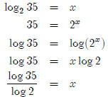
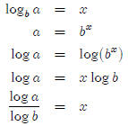
so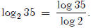 We can generalize this to get a formula for evaluating logs to

different bases.

So, in general, 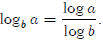This comes in handy at times.

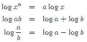
Lesson 6: Log rules for products and quotients

There are really just three rules that we need to pay attention here. They just seem a bit
strange so pay careful attention to what they say and what they don’t say.

The first rule, we’ve used a lot in solving exponential equations, so you should be fairly
used to it by now. The other two are new, but they’re important to learn. Let’s look at
why these are true.

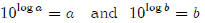
Why is ?

By definition,

Lesson 6: Log rules for products and quotients (Lesson Notes)

Raise both sides to the "a" power.

Use the laws of exponents to simplify.

Take the log of both sides.

Why is log ab = log a + log b?

By definition,

Multiply the two equations

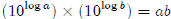
Use the laws of exponents

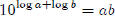
Take the log of both sides

Why is

By definition,

Divide the two equations

Use the laws of exponents

Take the log of both sides

Lesson 7: The importance of one-to-one when finding inverses (Lesson Notes)

Section: Square Roots and Inverses

Lesson 7: The importance of one-to-one when finding inverses

Many people like think that the inverse of y = x² is , which of course means that
the inverse of is y = x² This is almost true, but there is one very important catch
here that we need to pay attention to. Let’s start by thinking about what the inverse of
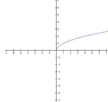
should look like. As we know, the graph of looks like this,

If we use what we know about the graphs of inverses and reflect this curve across the
diagonal line, y = x, we get this,

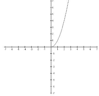
This looks something like the graph of f(x) = x², but it’s only half the parabola. We
can write this function as "f(x) = x² , x ≥0.”

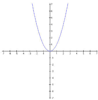
On the other hand, as you know, the graph of f(x) = x² looks like this.

Lesson 7: The importance of one-to-one when finding inverses (Lesson Notes)

If we use what we know about the graphs of inverse functions, and flip this across the
diagonal line, y = x, we get this,

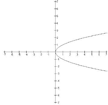
This is a problem because the graph shown above is not a function. We can tell that
because it doesn’t pass the vertical line test. This is a problem. We need our inverse
functions to be functions. If you think about it for a minute, it makes sense that the
inverse of a function will only pass the vertical line test if the original function passes the
horizontal line test. So in order to get y = x² to pass the horizontal line test, we restrict
the domain so we only have half of the parabola.

If a function passes the horizontal line test, we say that the function is one-to-one
(remember that it had to pass the vertical line test in order to be a function). A one-to-one

Lesson 8: Solving equations with square roots (Lesson Notes)

function has one y-value for every x-value (all functions have this property ) and one x-value
for every y-value. That’s why we call them one-to-one.

Very Important: In order to have an inverse, a function has to be one-to-one.

So if we want to talk about the inverse of y = x² , we have to do something like this.
The function y = x²  isn’t one-to-one, so we have to restrict the domain to x 0. In other
words, we define the function as 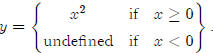. Sometimes we get lazy and
just write this as y = x², x≥ 0. The inverse of y = x², x≥ 0 is.

Going the other way is a little easier, the inverse of is y = x², x≥ 0.

We have to do similar restrictions to find the inverse of other functions that are not
one-to-one. This will become very important if you take trig.

Lesson 8: Solving equations with square roots

Solving equations with square roots is more or less what you would expect. You isolate
the radical, then square both sides. There is one important catch, however. When you
square both sides of an equation, you may create extraneous roots. In other words, you
may do all of your work correctly and still end up with a solution that does not work in
the original equation. Thus, it is very important to check your work to see if you
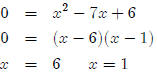
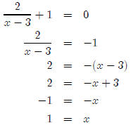
have extraneous roots. Let’s look at an example. Suppose we want to solve

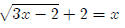
First we want to isolate the radical.

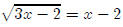
Then we square both sides.

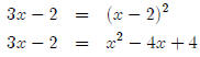
Now we have a quadratic equation, so we collect terms and set everything equal to zero,
then either factor or use the quadratic formula.

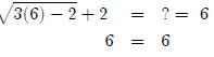
Now we need to check our answers in the original equation to see if we have any extraneous
roots. First we’ll check 6.

Lesson 9: Linear Inequalities (Lesson Notes)

So 6 checks out fine. Now we’ll try 1.

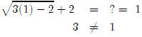
So 1 is an extraneous root. So our only solution is x = 6.

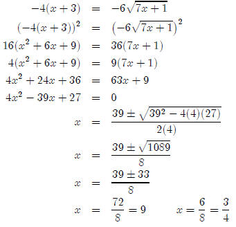
So what do we do if an equation has two radicals in it?

What if we have to solve something like,

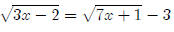
There’s really not much you can do but square both sides to get rid of one of the radicals,
then square both sides again. These problems tend to be a lot of work. Here we go

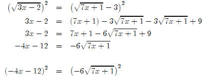
To make things easier, I’m going to factor −4 out of the left hand side.

Section: Inequalities

Lesson 9: Linear Inequalities

Solving inequalities is basically like solving equations. You just do the same thing to both
sides, and/or change things to an equivalent form, and you try to do this in an intelligent

Lesson 10: Solving non-linear inequalities by graphing (Lesson Notes)

way that eventually gets the variable you are solving for on one side of the equation and
everything else on the other side. There is only one small difference when you are solving
an inequality:

When you multiply or divide both sides by a negative, you have to reverse
the direction of the inequality.

This makes sense if you just look at some simple inequalities with numbers. For example,

5 < 9

This is a simple enough statement. But if I multiply both sides by −1, I get

−5 > −9

You have to reverse the direction of the inequality to still have a true statement. If you
think about where these numbers are on a number line, this should make sense.

Let’s look at a quick example

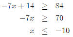
So the solution to this inequality is {x : x ≤−10}

Lesson 10: Solving non-linear inequalities by graphing

Let’s just start by looking at an example.

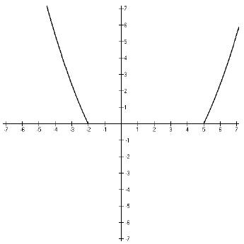
1. Example: Given the function f(x) represented by the following graph,

(a) determine the values of x for which f(x) is less than zero.

(b) determine the values of x for which f(x) is greater than zero.

Lesson 10: Solving non-linear inequalities by graphing (Lesson Notes)

The real key to being able to answer questions like this is being able to figure out which
part of the graph we are interested in. For Part (a) of the example question, we are
interested in the values of x for which the f(x) is less than zero. Since the value of f(x) is
that same as the y-value for any point on the graph, we simply look for the part(s) of the
graph that have negative y-values, which is this part,

Looking at the graph, it’s easy to see that the x-values that correspond with this part
of the graph are {x : −2 < x < 5}. Written in interval notation, it would be the interval
(−2, 5).

Note: We are using strict inequality (<, not ≤) because the problem asked us to find the
points for which f(x) is "less than zero." If the problem had read "less than or equal to
zero," we would have used ≤.

For Part (b) of the example question, we need to find the values of x for which f(x) is
greater than zero. That would be these parts of the graph.

Lesson 10: Solving non-linear inequalities by graphing (Lesson Notes)

The x-values that correspond to these parts of the graph would be {x : x < −2 or
x > 5}. In interval notation, this would be (− ∞,−2) ∪(5,∞ ).

Another example: Given the function f(x) represented by the following graph,

1. (a) determine the values of x for which f(x) is greater than or equal to zero.

Lesson 11: Inequalities involving quadratics (Lesson Notes)

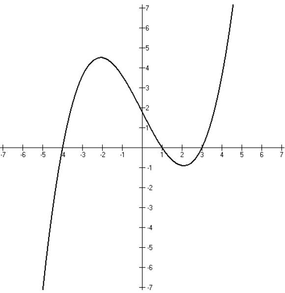
If you look at this and think about what we did in the previous example, you
should be able to figure out that the answer would be {x : −4≤ x ≤1 or x ≥3}.
In interval notation, [−4, 1] ∪[3,∞ ).

Lesson 11: Inequalities involving quadratics

The key to understanding how to solve inequalities involving quadratics or other polynomials
is to realize that these functions are continuous. This means that they don’t jump from
one point to the next without points in between. Continuous functions can’t go from being
less than zero to being greater than zero without being equal to zero at some point.

So here is our basic strategy for solving inequalities involving quadratics or other poly-
nomials.

• First, move everything to one side of the inequality so one side is equal to zero.

• Then change the inequality to an equation and find the x-values for which the function
is equal to zero. These points are the possible boundaries for your intervals.

• Then you need to figure out which intervals you want. The easiest way to do this is

Lesson 11: Inequalities involving quadratics (Lesson Notes)

to graph the function and use what you know about solving inequalities by looking
at graphs.

— Note: if you do this on a test or quiz, you need to draw a rough sketch
of the graph.

An example: Solve for x.

• 4x² + 5x − 6 ≥0

First we change the inequality to an equation.

4x² + 5x − 6 = 0

Now we need to solve the equation. Looking at the diamond puzzle, I think it will
factor, so we have.

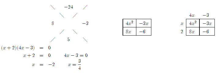
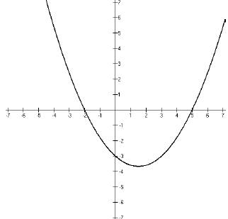
So we know that the possible boundaries of our intervals are x = −2 and x =3/4
So. now we graph the function and we see that the graph looks like this,

Lesson 11: Inequalities involving quadratics (Lesson Notes)

So our answer is {x : x < −2 or x >3/4}. In interval notation, this would be

(− ∞,−2) ∪(3/4, ∞).

Another example: Solve for x

• x³ − 6x²+ 9x ≤0

First we write this as an equation and factor

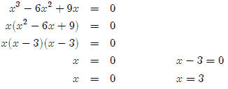
Now we look at the graph.

Lesson 12: Inequalities involving rational functions (Lesson Notes)

What we notice here is that the graph crosses the x-axis at x = 0, but it just touches
the x-axis at x = 3. So our solution is {x : x ≤0 or x = 3}. In interval notation,
(− ∞, 0]∪ [3, 3].

Lesson 12: Inequalities involving rational functions

Inequalities involving rational functions are tricky because rational functions are not continuous.
This means that it is possible for f(x) to go from being less than zero to being
greater than zero without ever actually being equal to zero. We need to pay attention
to this when we are working with inequalities involving rational functions. The strategy
for solving inequalities of this type is, however, very similar to the strategy we used when
working with polynomials. We just have to look for discontinuities as well.

So here is our basic strategy for solving inequalities involving rational functions.

• First, move everything to one side of the inequality so one side is equal to zero.

• Then change the inequality to an equation and find the x-values for which the function
is equal to zero.

• Then find all discontinuities (breaks in the domain)

• The zeroes and the discontinuities are the points that are possible boundaries for your
intervals.

• Then you need to figure out which intervals you want. The easiest way to do this is
to graph the function and use what you know about solving inequalities by looking
at graphs.

Lesson 12: Inequalities involving rational functions (Lesson Notes)

— Note: if you do this on a test or quiz, you need to draw a rough sketch
of the graph.

An example: Solve for x

First we find the values for which the function is equal to zero.

Next, we notice that the function has a discontinuity at x = 3. Putting this together
with the root we just found, the possible boundaries of our solution are x = 1 and x = 3.
So now we need to look at the graph.

Looking at the graph and putting this together with what we have figured out, we can
see that our solution is {x : x ≤1 or x > 3}. In interval notation, (−∞ , 1] ∪(3, ∞).
Notice that 1 is included in our solution, but 3 is not. If you look at the graph and think
about what is happening, you should be able to figure out why.

Lesson 13: Solving inequalities with absolute value (Lesson Notes)

Lesson 13: Solving inequalities with absolute value

Solving inequalities involving absolute value is basically the same as solving inequalities
involving quadratics. The absolute value function is continuous so we don’t have to worry
about discontinuities. So we use the same strategy we used on inequalities involving
quadratics.

• First, move everything to one side of the inequality so one side is equal to zero.

• Then change the inequality to an equation and find the x-values for which the function
is equal to zero. These points are the possible boundaries for your intervals.

• Then you need to figure out which intervals you want. The easiest way to do this is
to graph the function and use what you know about solving inequalities by looking
at graphs.

— Note: if you do this on a test or quiz, you need to draw a rough sketch
of the graph.

The only problem you might have is that you might not know how to put the absolute
value function in your calculator. It’s under the MATH menu and it looks like this, "abs."
So if you wanted to put |2x + 3| into your calculator, it would look like "abs(2x + 3).

Section: Conics

Lesson 14: Parabolas

This lesson isn’t that important. Don’t loose sleep over it.

Lesson 15: Circles

We start this lesson by talking about the distance formula. You should be familiar with the
Pythagorean theorem for right triangles, a² +b² = c². If you translate this to a coordinate
grid and you are trying to calculate the distance, d, between two points, the Pythagorean
theorem would be (Δ x)² + (Δ y)² = d². If we take the the square root of both sides, this
becomes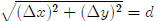

To relate this formula to the coordinates of the points involved, lets assume that we
want to find the distance between two points A = (x₁, y₁) and B = (x₂, y₂). In this case,
Δx = x₂ − x₁ and Δy = y₂ − y₁ so our formula becomes

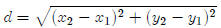
This is usually referred to as "the distance formula" for obvious reasons and it is fairly
important.

Lesson 15: Circles (Lesson Notes)

A circle centered at the origin is just all the points that are the same distance from the
origin. We call this distance the radius and usually notate it with r. So the equation for
a circle at the origin is

which is usually written as x² + y² = r²

Of course not every circle is centered at the origin. Let’s let A = (h, k) be the center of
our circle and B = (x, y) be any point on the circle. Knowing that the distance between
the center and any point on the circle is always the constant r, we get

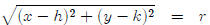
which is usually written as (x − h)² + (y − k)² = r²

This is the general equation for a circle centered at (h, k) with radius r.

Notice that both h and k have negative signs in front of them, whereas in other equations
such as the vertex form of a parabola, y = a(x − h)² + k, the h had a negative in front of
it and the k did not. This makes sense if you think about the fact that in the vertex form
of a parabola, y and k are on opposite sides of the equation, while in the general equation
for the circle, they are on the same side.

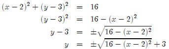
So how do we graph a circle on our calculator? For example, how do we graph (x −
2)²+(y−3)² = 16? Just looking at the equation and applying what we know about circles,
we know that this is a circle centered at (2, 3) with a radius of 4. To graph this on our
calculator, we’re going to have to solve this equation for y.

Since we don’t have a ± key on the calculator, we have to split this into two equations.
So what we put in the calculator should look something like this.

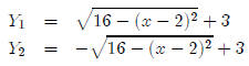
If you put these two equations in your calculator and graph them, you’re going to get
something that looks more like an ellipse than a circle. That is because the calculator
screen isn’t square so the scales in the x-direction and the y-direction are different. To get
something that looks more like a circle, you need to go to ZOOM and hit Zsquare, with
will make the scales the same in both directions.

Lesson 16: Ellipses (Lesson Notes) 23

Lesson 16: Ellipses

You can think of an ellipse as a circle that has been stretched in one direction. The standard
form that I will use for an ellipse is

where c² = la² − b²l

This is basically the same formula that you have on your formula sheet with a few minor
changes. If you use the version on the formula, you have to remember that a² needs to be
bigger than b². I find it easier to just put a² under the x, and b² under the y and then
take the absolute value to find c². You’ll get the same answer either way. An ellipse in
this form has its center at (h, k).It stretches to the left and right a units from the center,
and it stretches up and down b units from the center. We’ll talk about c in a bit. First,
let’s look at an example.

Example: For the ellipse given by the equation

• Make a sketch of the graph of the ellipse

• Find the center

• Find the length of the major axis

• Find the length of the minor axis

• Find the vertices

Since this equation is already in standard form, we can tell a lot just by looking at it.
We know that the ellipse is centered at (3,−1), that it stretches to the left and right 2 units
from the center and up and down three units from the center. So we can sketch our graph;
it looks like this.

Lesson 16: Ellipses (Lesson Notes)

The distance across the ellipse in from right to left is 2a, which in this ellipse is 4. The
distance up and down is 2b, which in this ellipse is 6. The major axis is the longer of these
two distances and the minor axis is the smaller. So for our ellipse,

• The length of the major axis is 6

• The length of the minor axis is 4

• The vertices (also sometimes called the foci) are two points inside the ellipse on the
major axis. The distance c is the distance from the center to each vertex. In this
ellipse,

So the vertices are located at (3, −1 + ) and (3, −1 − ). If we use decimals,
the vertices will be at (3, 1.236) and (3,−3.236).

So what do we do if the equation of our ellipse is not already in standard form? In this
case we have to complete the square (twice). Let’s look at an example.

Completing the square example:
Put the equation 9x² − 54x + 4y² + 8y + 49 = 0 into standard form.

OK, so how do we know this equation is an ellipse? It is an ellipse because it has an
x² term in it, a y² term in it, and both the x² term and the y² term are positive. If either

Lesson 17: Hyperbolas (Lesson Notes)

the x² term or the y² term were negative, we would have a hyperbola, which we will talk
about later. It could be a circle (technically a circle is a type of ellipse), but we know it
isn’t because the coefficients of the x² term and the y² term are different. So we need to
complete the square.

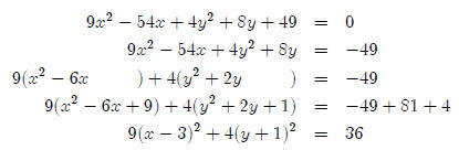
So far, this has been more or less like completing the square for a parabola, we just had
to do it twice. Now we have to make the right hand side equal one by dividing everything
by 36.

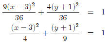
Which is in standard form. (Note that this is the equation that we used above.)

Lesson 17: Hyperbolas

Note: Cohen (2003) has a pretty good section about hyperbolas. See especially
pp. 670-674.

The equation for a hyperbola is just like the equation for an ellipse, except that there
is a negative sign between the two fractions. There are two forms of the equation for a
hyperbola.

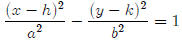or

The center of the hyperbola is at (h, k). The asymptotes (hyperbolas have slant asymptotes)
go through the center and have slope ±b/a. Graphing a hyperbola takes a little
work, but there are some tricks that make it not too bad. Let’s look at an example.
Example: Graph

• First we notice that the center of the hyperbola is at (3, 1), so we find that point on
our graph.

• Then we count a spaces to the left and right and make a mark. For our hyperbola,
that will be 4 spaces left, 4 spaces right, 2 spaces up, and 2 spaces down. So we have
this.

Lesson 17: Hyperbolas (Lesson Notes)

• Now we mark the corners of a box made by our marks. Then we draw in the diagonals
of the box as dotted lines. These will be the asymptotes of our hyperbola.

• Now we need to figure out if our hyperbola goes up and down or right and left. The
rule is that the vertices go in the direction of the positive term and the empty space
goes in the direction of the negative term. So for our parabola, the x-term is positive
and the y-term is negative, so our vertices go on our box to the left and right of the
center. Then we can draw in the hyperbola. In comes down an asymptote, curves
and touches the vertex, and then goes out the other asymptote. It looks like this.

Lesson 18: Polynomial long division. The commonly known way of dividing polynomials. (Lesson Notes)27

Section: Misc Stuff

Lesson 18: Polynomial long division. The commonly known way of dividing
polynomials.

The book (Cohen, 2003) does a pretty good job of explaining polynomial long division on
pp. 570 and 571

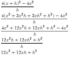
Lesson 19: Difference quotient

The difference quotient is used to estimate the slope of the tangent to a curve at a point. It
is very important in calculus. Right now, we’re not going to worry too much about where
it comes from, but we need to learn to work with it and simplify it. The difference quotient
for any function f(x) is,

You should be able to simplify the difference quotient for the following types of functions

• Quadratic polynomials such as f(x) = 3x² − 2x + 5

• Simple cubic polynomials such as f(x) = 4x³

I will do an example of each

Lesson 19: Difference quotient (Lesson Notes)

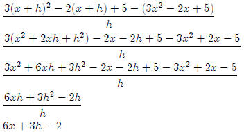
Quadratic example: Simplify the difference quotient for f(x) =
3x² − 2x + 5

First note that

f(x + h) = 3(x + h)² − 2(x + h) + 5

So the difference quotient is

Simple cubic example: Simplify the difference quotientfor f(x) =
4x³

First note that

f(x + h) = 4(x + h)³

So the difference quotient is

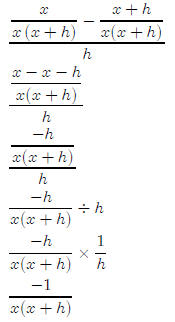
Example1/x: Simplify the difference quotient for f(x) =1/x

The difference quotient is fairly straightforward

Lesson 20: Non-linear systems (Lesson Notes)

So we need to get a common denominator on top and simplify

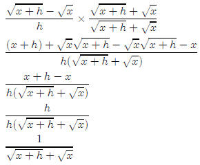
Square root example: Simplify the difference quotientfor f(x) =


This one is fairly hard. (Hint: It might be a good extra credit question)
Once again, the difference quotient is fairly simple

There is a trick to simplifying this. We multiply top and bottom by

Lesson 20: Non-linear systems

Generally, the best way to solve a non-linear system is substitution. Sometimes, it is
difficult or impossible to solve a system using substitution, so the only way to do it is to
graph the two equations and find the intersection of the two graphs.

Lesson 21: Binomial Theorem revisited (Lesson Notes)

Lesson 21: Binomial Theorem revisited

Although we didn’t use the term "binomial theorem," we actually talked about the binomial
theorem when we learned to use Pascal’s triangle to expand expressions like (x + y)⁴. In
this lesson, we are learning to find the coefficients of a term without using the triangle.

Before we talk about the binomial theorem itself, we need to learn about the "choose
numbers." These are the numbers that are in Pascal’s triangle, but it is possible to calculate
them directly without doing the whole triangle. An example of a "choose number" is
. . This should be read as "5 choose 3." It gets this name because it is the number
a different ways you can choose 3 things from a group of 5 things if order doesn’t matter..
So if you want to calculate "5 choose 3," you just get your calculator, put in 5, then to
to MATH, PRB, and select   then put in 3 and hit ENTER. You should get 10. If
you look at Pascal’s triangle, you will see that 10 is the third term in the 5th row of the
triangle. This works in general. So is the 2nd entry in the 6th row,  11 is
the 4th entry in the 11th row.

There is another, more traditional notation that was the standard notation before calculators.
Using this notation, "5 choose 3" is written as. If we want to write "6
choose 2" using this notation, we would write.
 

The binomial theorem looks pretty intimidating, but once you figure out what it actually
means, it’s not that bad. Here is the binomial theorem. It’s not something you need to
memorize. It’s on the formula sheet.

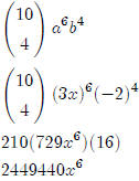
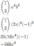
So how do we use this awkward looking beast. Let’s say we wanted to know (for
some reason, I really don’t know why we would want to know this) the fourth term in the
expansion of (x+y)¹². We would look at the pattern in the theorem and see that the fourth
term would have the form Since we know that n = 12 for this question, we

have

We get out our calculator and put in and get 220. So we have

220a⁹b³

Another example:

Lesson 22: More word problems (Lesson Notes)

Find the fifth term in the expansion of (3x − 2)¹⁰

One more example:

Find the fourth term in the expansion of (2x − 1)⁷

Lesson 22: More word problems

One of the challenges of this lesson is getting used to some new language. Let’s look at an
example:

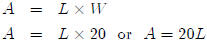
The width of a rectangle is 20 inches.
(a) Express the area of the rectangle as a function of the length.
(b) Express the length of the rectangle as a function of the area.

So what is this question asking you to do when it asks you to "Express the area of the
rectangle as a function of the length?" It’s asking you to write an equation where one side
of the equation is the area (the thing we’re expressing) and the other side is a mathematical
expression where the only variable is the length. In this problem, it’s pretty easy. We
know that the area of a rectangle is length × width, and we know that the width of the
rectangle is 20 inches. So

There, we’re done with Question (a). We have expresses area in terms of length. In
other words, we have expressed area as a functin of length. If you give me a length, I can
plug it into the right side of this equation and figure out what the area must be. This is
what we mean by expressing area in terms of length.

Lesson 22: More word problems (Lesson Notes)

But what about Question (b)? Question (b) asks us to express the length as a function
of the area. This means we need to get length all by itself on one side. The easiest way
to do this is to start with what we already have and solve for L.

We’re done. We have now expressed length as a function of area.

Let’s look at another example.

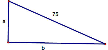
A right triangle has a hypotenuse with length 75.
(a) Express the length of one leg as a function of the length of the other leg.
(b) Express the area as a function of one of the legs.

Anytime you’re working a problem like this, it helps to draw a picture. Here’s the
picture I drew (with a little help from geometer sketchpad)

Now we need to remember what we know about right triangles. I seem to remember
something related to a Greek guy named Pythagorus. Let’s see, Pythagorean Theorem,

a² + b² = c²

In this problem, this translates to

a² + b² = 75²

So if I could solve this for one of the sides in terms of the other, I’d be done with Question
(a). Let’s give it a shot.

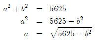
So we’re done with question (a).
If you’re paying attention, you may wonder why I didn’t put a "±” in front of the
radical. In the context of this problem, ”a” represents the length of one of the sides, and
it doesn’t make sense for a length to be negative.

For question (b), we need to remember the formula for the area of a triangle. Hopefully,
you remember that the area of a triangle is where b is the base of the triangle and h is

Lesson 23: Still more word problems (Lesson Notes)

the height. Since we have a right triangle, the base and height are just the lengths of the
two legs. So the area of our triangle is

which we can write as

But aren’t done yet. Question (b) asked us to "find the area as a function of one of
the legs." Right now, we have the area as a function of both of the legs. So we need to
figure out a way to write this in terms of one of the legs. If we look back at our solution
to Question (a), we can see that we have an equation that relates the two legs. So we can
do a substitution.

But from (a), we know

So which we can write as
 

So now we’re done. We have expressed the area as a function of one of the legs. In
other words, we have come up with an equation that has the area on one side, and an
expression involving one of the legs on the other side.

All of the problems in this section are similar. I’m not saying that they’re all easy, but
they all ask you to "express this as a function of that."

Lesson 23: Still more word problems

In this lesson, we will be finding the maximum or minimum values of a function. Usually
(but not always), these functions will be quadratics. If the function is a quadratic, the
maximum or minimum will be at the vertex. There are three ways we can find the vertex.

• If the equation is already in vertex form, we can just read it from the equation. Of
course, we can always complete the square to put the equation in vertex form, but
usually we don’t need to do that much work.

• We can use our calculator, graph the function, and then use the CALC menu to find
the maximum or minimum value. You have to set your Left Bound and Right Bound,
just like you did when you used the calculator to find zeroes, but it’s pretty easy to
figure out.

• We can find the vertex using a nifty new formula that we’re learning in this lesson.
If a quadratic is written in standard form, y = ax² +bx+c, then the x-coordinate of
the vertex is given by

Notice that this is just the quadratic formula when the discriminant (the part under
the radical) is equal to zero. If you scratch your head and think a bit, you can
probably figure out why is makes sense for this to be the x-coordinate for the vertex.
Whether or not you figure out why it makes sense, you can use this formula to find
the vertex of a parabola without having to complete the square.

Lesson 23: Still more word problems (Lesson Notes)

Let’s look at an example. Let’s say we need to find the maximum or minimum of the
following function and identify whether it is a maximum or a minimum.

y = 3x² + 24x + 17

If you really want to complete the square, don’t let me talk you out of it, but I’m going to
use our nifty new formula.

So that gives us our x-value. How do we find the y-value? The same way we always
do, by plugging in x.

So our vertex is at (−4,−31). Now, is this a maximum or a minimum? Think about what
the graph looks like. Does it open up or down? You should be able to figure out that it
opens up, which means that this point is a minimu. So this function has a minumum value
of −31 that occurs when x = −4.

The word problems in this section are the same problems we did in the previous lesson,
only now we have to find a maximum or a minimum. So you should already have the
functions you need, you just need to find the max or min. Many of them are quadratics,
so you can use the handy formula above or use your graphing calculator. For the functions
that are not quadratics, you’ll need to use your graphing calculator.